Electromagnetic Waves, Antennas, and RF: Spatial Derivatives of Fields - Gradient, Divergence, and Curl

EM01 introduced scalar and vector fields, and EM02 developed the vector algebra needed to describe their magnitude, direction, projection, and transverse wave geometry. The next step is to ask how a field changes from one nearby point in space to another.

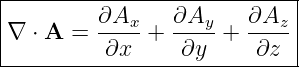
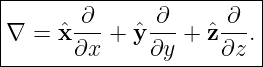
For an ordinary function of one variable, the derivative answers that question. For a field in three-dimensional space, there is more than one possible kind of spatial change. The three most important first-order differential operations are

|----------------------------------| -gradient,----divergence,-----curl.|

(1)

These operations are the mathematical language in which Maxwell’s equations will eventually be written. EM03 develops them before Maxwell’s equations appear, so the later physics will not be obscured by unfamiliar vector calculus [1, 2, 3, 4].

1 From an ordinary derivative to a spatial derivative

For a function of one variable,

f = f (x),

(2)

the derivative

-df- dx

(3)

measures the local rate of change of f as x changes.

In three-dimensional space, a scalar field depends on several coordinates:

ϕ = ϕ(x, y,z).

(4)

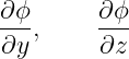
Changing x while holding y and z fixed gives the partial derivative

|----| |∂ϕ- | |∂x .| ------

(5)

Similarly,

∂ϕ-, ∂ϕ- ∂y ∂z

(6)

measure local change in the other coordinate directions.

Partial derivatives are therefore ordinary local slopes taken along selected coordinate directions.

1.1 Units of a spatial derivative

If ϕ has units [ϕ], then

[ ] ∂ϕ- [ϕ] ∂x = m .

(7)

Every spatial derivative introduces one inverse power of length. This dimensional fact is a useful check throughout vector calculus.

2 The nabla operator

In Cartesian coordinates it is convenient to collect the three spatial derivative directions into the differential operator

|------------------------| |∇ = ˆx-∂- + ˆy-∂- + ˆz-∂-.| -------∂x-----∂y-----∂z---

(8)

The symbol ∇ is pronounced “del” or “nabla.”

It resembles a vector, but it is not an ordinary physical vector. Its components are derivative operations. What ∇ produces depends on what follows it and on whether it is used directly, dotted into a vector field, or crossed with a vector field.

The three central constructions are

|----------------------------| |∇ ϕ, ∇ ⋅ A, ∇ × A. | -----------------------------

(9)

Their input and output types differ.

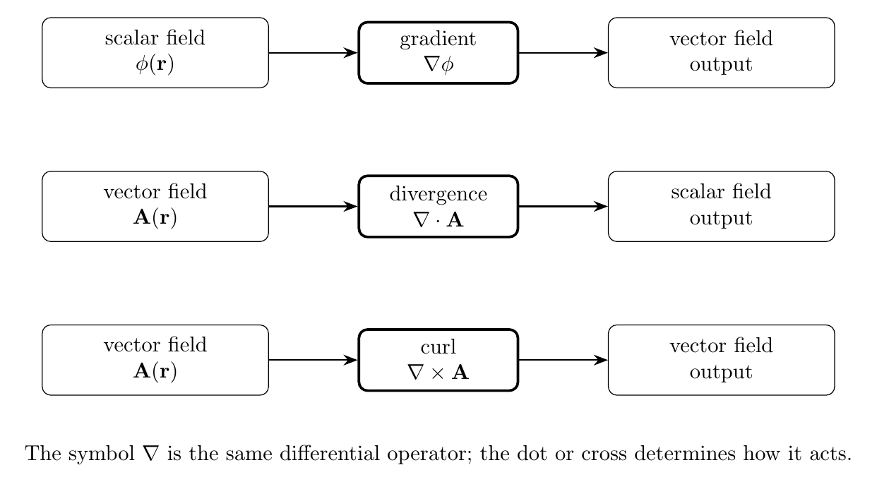
Figure. gradient maps a scalar field to a vector field, divergence maps a vector field to a scalar field, and curl maps a vector field to another vector field.

3 Gradient of a scalar field

Let

ϕ = ϕ(x, y,z).

(10)

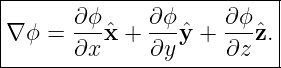
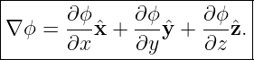
The gradient is

|--------------------------| |∇ ϕ = ∂-ϕˆx + ∂ϕyˆ+ ∂ϕ-ˆz.| -------∂x------∂y-----∂z---|

(11)

The input ϕ is a scalar field. The output ∇ϕ is a vector field.

Each component tells how rapidly ϕ changes in one coordinate direction.

For example, if

ϕ(x,y, z) = x2 + 2y2 + 3z,

(12)

then

	= 2x,	(13)
	= 4y,	(14)
	= 3,	(15)

|----------------------| |∇ϕ = 2xˆx + 4y ˆy + 3ˆz.| ------------------------

(16)

The gradient can vary from point to point even when the original scalar field is smooth.

4 Geometric meaning of the gradient

The gradient has two closely related geometric meanings:

it points in the direction of the fastest local increase of the scalar field;
it is normal to a surface on which the scalar field is constant.

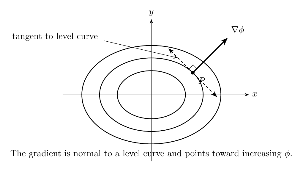
Figure. Level curves represent constant values of a scalar field. The gradient is perpendicular to the local tangent of a level curve and points toward increasing field value.

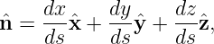
To derive the first statement, imagine moving through space along a path r(s), where s is distance along the path. Let the unit tangent to the path be

ˆn = dr-. ds

(17)

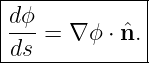
The chain rule gives

(18)

But

ˆn = dxxˆ+ dyyˆ+ dzˆz, ds ds ds

(19)

|-------------| d ϕ | --- = ∇ ϕ ⋅ ˆn.| -ds------------

(20)

This is the directional derivative of ϕ along n.

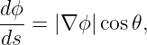
Using the dot product,

dϕ ---= |∇ ϕ|cos 𝜃, ds

(21)

where 𝜃 is the angle between ∇ϕ and n.

The largest possible value occurs when

𝜃 = 0,

(22)

so the direction of fastest increase is the direction of the gradient.

5 Why the gradient is normal to a level surface

Suppose a path lies entirely on a level surface

ϕ = constant.

(23)

Along that path,

dϕ-= 0. ds

(24)

Therefore

∇ ϕ ⋅ˆt = 0,

(25)

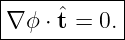
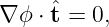
where t is any tangent direction to the level surface.

Hence

--------------------- ∇ ϕ ⊥ level surface. | ---------------------

(26)

This result will later connect naturally with plane-wave phase. Surfaces of constant phase are wavefronts, and the wave vector is normal to those surfaces.

6 Divergence of a vector field

Now consider a vector field

A = A ˆx + A ˆy + A ˆz. x y z

(27)

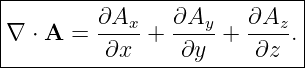
The divergence is obtained by taking the dot product of ∇ with A:

|----------------------------| | ∂Ax ∂Ay ∂Az | |∇ ⋅ A = ---- + ----+ ----.| ----------∂x-----∂y------∂z---

(28)

The input is a vector field. The output is a scalar field.

Divergence measures local net outward flux density: whether, in a very small neighborhood, more field flux tends to leave than enter.

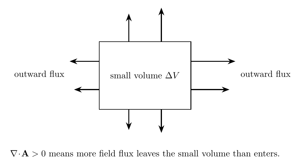
Figure. Positive divergence corresponds locally to net outward flux from a small volume. Negative divergence corresponds to net inward flux.

7 Deriving divergence from a small box

Take a small rectangular box with side lengths

Δx, Δy, Δz

(29)

and volume

ΔV = Δx Δy Δz.

(30)

Consider the two faces perpendicular to the x direction. The net outward contribution from those faces is approximately

[ ( ) ( ) ] Δx-- Δx-- Ax x + 2 − Ax x − 2 Δy Δz.

(31)

For sufficiently small Δx,

( ) ( ) Δx-- Δx-- ∂Ax- Ax x + 2 − Ax x − 2 ≈ ∂x Δx.

(32)

Thus the x-face contribution becomes

∂Ax ----ΔV. ∂x

(33)

The same argument for the y and z faces gives total net outward flux

( ∂Ax ∂Ay ∂Az ) Δ Φ ≈ ----+ ----+ ---- ΔV. ∂x ∂y ∂z

(34)

Therefore

|------------------| |Δ Φ ≈ (∇ ⋅ A )ΔV.| -------------------

(35)

This is the local physical meaning of divergence.

8 Interpreting the sign of divergence

At a point,

∇⋅ A	> 0	indicates local net outward flux,	(36)
∇⋅ A	< 0	indicates local net inward flux,	(37)
∇⋅ A	= 0	indicates zero local net flux to first order.	(38)

The word “source” is often used for positive divergence and “sink” for negative divergence.

However, zero divergence does not mean the vector field is zero. It means only that the local first-order balance of outward and inward flux is zero.

9 Curl of a vector field

Divergence measures local net outflow. Curl measures a different geometric property: local circulation.

For

A = Ax ˆx + Ay ˆy + Azˆz,

(39)

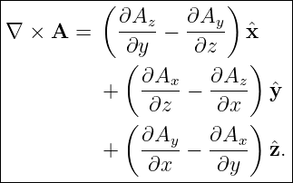
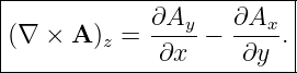
the curl is

|------------------------------| | ( ∂Az ∂Ay ) | |∇ × A = ----− ---- ˆx | | ∂(y ∂z ) | | ∂Ax- ∂Az- | | + ∂z − ∂x ˆy | | ( ) | | + ∂Ay- − ∂Ax- ˆz.| | ∂x ∂y | -------------------------------

(40)

The input is a vector field, and the output is another vector field.

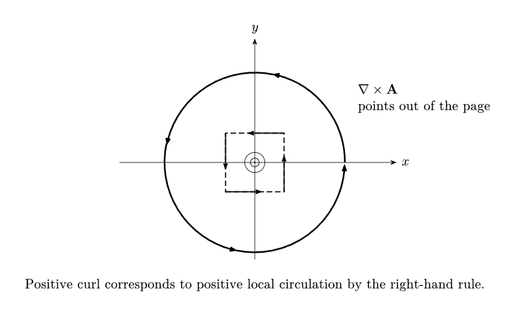
Figure. Curl measures local oriented circulation. The direction of the curl vector follows the right-hand rule.

10 Deriving one component of curl from a small loop

Consider a small rectangular loop in the xy plane. Traverse it counterclockwise when viewed from +z.

The circulation around the loop is

∮ A ⋅ dℓ.

(41)

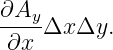
To first order, the two horizontal edges contribute

∂Ax- − ∂y Δx Δy,

(42)

while the two vertical edges contribute

∂Ay ----Δx Δy. ∂x

(43)

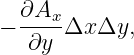
Adding them gives

∮ ( ) A ⋅ dℓ ≈ ∂Ay- − ∂Ax- Δx Δy. ∂x ∂y

(44)

Therefore

|------------------------| (∇ × A )z = ∂Ay- − ∂Ax-.| --------------∂x-----∂y---

(45)

The other two components follow from the same argument applied to loops in the yz and zx planes.

This establishes the local interpretation

|--------------circulation-around--a-small-loop--| |(∇ × A ) ⋅ ˆn ≈-------------------------------.| -----------------------area-of the-loop---------

(46)

11 Curl and local rotation

A useful model field is

A = − Ωy ˆx + Ωx ˆy.

(47)

Its divergence is

∇ ⋅ A = 0 + 0 + 0 = 0.

(48)

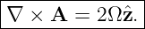
But its curl is

∇× A	= z	(49)
	= 2Ωz.	(50)

Thus

|--------------| -∇-×-A--=-2Ω-ˆz.-

(51)

This field circulates locally even though it has zero divergence.

For a rigid-body velocity field, the curl is twice the angular-velocity vector. That factor of two is specific to the relation between curl and rigid rotation; curl itself should not generally be identified directly with angular velocity.

12 Gradient, divergence, and curl answer different questions

The three operations should not be treated as interchangeable versions of “taking a derivative.”

For a scalar field ϕ,

|-------------------------------------------------------------------| ∇ ϕ asks: in which direction does the scalar increase most rapidly?| --------------------------------------------------------------------

(52)

For a vector field A,

|------------------------------------------------------| -∇-⋅ A--asks:-is there-local net-outward-or-inward-flux?--

(53)

and

|------------------------------------------------| |∇ × A asks: is there local oriented circulation?| --------------------------------------------------

(54)

Their output types are different:

scalar	vector,	(55)
vector	scalar,	(56)
vector	vector.	(57)

13 Gradient of a plane-wave phase

EM02 introduced the three-dimensional plane-wave phase

𝜃(r,t) = k ⋅ r − ωt.

(58)

Write

k = kxˆx + kyˆy + kzˆz.

(59)

Then

𝜃 = kxx + kyy + kzz − ωt.

(60)

Taking the spatial gradient,

∇𝜃	= k_xx + k_yy + k_zz	(61)
	= k.	(62)

Therefore

|--------| -∇-𝜃 =-k.-

(63)

This result gives a precise differential meaning to the statement from EM02 that the wave vector is normal to constant-phase surfaces.

14 Gradient of a scalar plane wave

Consider

ψ (r,t) = ψ0cos(k ⋅ r − ωt).

(64)

Let

𝜃 = k ⋅ r − ωt.

(65)

Using the chain rule,

∇ ψ = − ψ0 sin 𝜃 ∇𝜃.

(66)

Since ∇𝜃 = k,

|--------------------------| ∇ ψ = − ψ0k sin(k ⋅ r − ωt). ----------------------------

(67)

The gradient of this scalar plane wave is therefore parallel or antiparallel to the wave vector, except at points where the gradient vanishes.

15 A vector plane wave can have zero divergence but nonzero curl

Now consider the simple vector field

|--------------------------| E (z,t) = ˆxE0 cos(kz − ωt).| ----------------------------

(68)

Its components are

E = E cos(kz − ωt ), E = 0, E = 0. x 0 y z

(69)

The divergence is

∇⋅ E

(70)

Although E_x varies with z, it does not vary with x. Therefore

∂Ex- = 0, ∂x

(71)

and

|----------| -∇-⋅ E-=-0.-

(72)

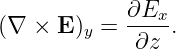
The curl, however, contains

∂Ex- ∂Ez- (∇ × E )y = ∂z − ∂x .

(73)

Hence

|------------------------------| |∇ × E = − kE sin(kz − ωt)ˆy. | ---------------0---------------

(74)

This example is important because it separates the ideas clearly:

|----------------------------------------| -∇-⋅ E-=-0--does-not-imply---∇--×-E-=--0.|

(75)

Later Maxwell equations will relate curls of electric and magnetic fields to time variation. EM03 does not use those equations yet; it only establishes the Differential Geometry needed to read them.

16 Worked Example 1: compute a gradient

Let

ϕ (x,y) = 3x2 + 2xy + y2.

(76)

Find ∇ϕ and evaluate it at

(x,y) = (1,− 1).

(77)

The partial derivatives are

	= 6x + 2y,	(78)
	= 2x + 2y.	(79)

Therefore

∇ ϕ = (6x + 2y)ˆx + (2x + 2y)ˆy.

(80)

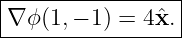
At (1,−1),

∇ϕ	= [6(1) + 2(−1)]x + [2(1) + 2(−1)]y	(81)
	= 4x.	(82)

Thus

|----------------| |∇ϕ (1,− 1) = 4ˆx.| ------------------

(83)

The scalar field increases most rapidly locally in the +x direction.

17 Worked Example 2: directional derivative and a level curve

Let

ϕ (x,y) = x2 + 2y2.

(84)

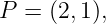
At the point

P = (2,1),

(85)

the gradient is

∇ ϕ = 2xˆx + 4y ˆy = 4ˆx + 4yˆ.

(86)

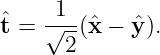
Choose the unit tangent direction

-1-- ˆt = √ -(ˆx − yˆ). 2

(87)

The directional derivative is

	= ∇ϕ ⋅t	(88)
	= (4x + 4y) ⋅(x −y)	(89)
	=	(90)
	= 0.	(91)

Thus

|----------| ∇-ϕ-⋅ˆt-=-0.-

(92)

The chosen direction is tangent to the level curve through P, while the gradient is normal to it.

18 Worked Example 3: compute divergence

Let

A = 2x ˆx − yˆy + 3zˆz.

(93)

Then

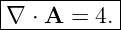
∇⋅ A	= + +	(94)
	= 2 − 1 + 3	(95)
	= 4.	(96)

Therefore

|----------| ∇ ⋅ A = 4.| ------------

(97)

The divergence is positive everywhere, so the field has local net outward flux everywhere in this model.

19 Worked Example 4: a divergence-free rotational field

Let

A = − 3yˆx + 3xyˆ.

(98)

The divergence is

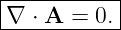
∇⋅ A	= +	(99)
	= 0 + 0	(100)
	= 0.	(101)

Thus

|----------| ∇ ⋅ A = 0.| ------------

(102)

But the field need not be spatially constant or zero. It can circulate while maintaining zero local net outflow.

20 Worked Example 5: compute curl

For the same field,

A = − 3yˆx + 3xyˆ,

(103)

only the z component of curl is nonzero:

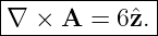
(∇× A)_z	= −	(104)
	= 3 − (−3)	(105)
	= 6.	(106)

Therefore

|----------ˆ-| ∇--×-A--=-6z.-

(107)

The positive z direction corresponds to counterclockwise local circulation when viewed from +z.

21 Worked Example 6: gradient of a plane wave

Let

ψ (r,t) = 4cos(2x + 3z − ωt).

(108)

The wave vector is

k = 2ˆx + 3ˆz.

(109)

Using the plane-wave gradient result,

∇ ψ = − 4(2ˆx + 3ˆz)sin(2x + 3z − ωt).

(110)

Thus

|------------------------------------| ∇ ψ = (− 8 ˆx − 12ˆz)sin(2x + 3z − ωt). --------------------------------------

(111)

At phase

2x + 3z − ωt = π-, 2

(112)

we obtain

|------------------| -∇-ψ-=-−-8ˆx-−-12-ˆz.|

(113)

The gradient points opposite k at that phase because the sine factor is positive and the derivative of cosine contributes a minus sign.

22 Worked Example 7: divergence and curl of a transverse wave field

Let

E (z,t) = ˆxE0 cos(kz − ωt).

(114)

Since

Ex = E0 cos(kz − ωt)

(115)

depends on z, not x,

∂Ex- ∂x = 0.

(116)

The other components vanish, so

|----------| -∇-⋅ E-=-0.-

(117)

For the curl,

∂E (∇ × E)y = ---x . ∂z

(118)

Therefore

∇× E

= −kE₀ sin(kz − ωt)y.

(119)

Hence

|------------------------------| |∇ × E = − kE sin(kz − ωt)ˆy. | ---------------0---------------

(120)

This is an early example of why divergence and curl encode genuinely different information about the same field.

23 Common mistakes

Mistake: treating ∇ as an ordinary physical vector. It is a differential operator whose components contain partial derivatives.
Mistake: forgetting that gradient acts on a scalar field and produces a vector field.
Mistake: assuming divergence differentiates every component with respect to every coordinate. In Cartesian form, divergence pairs A_x with x, A_y with y, and A_z with z.
Mistake: thinking zero divergence means the vector field is zero. A circulating field can have zero divergence.
Mistake: thinking curl merely means that drawn field lines look curved. Curl measures local oriented circulation density.
Mistake: confusing ∇⋅ A, which is a scalar, with ∇× A, which is a vector.
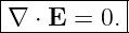
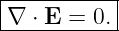
Mistake: assuming ∇⋅ E = 0 implies ∇× E = 0. These are independent local properties.
Mistake: forgetting units. Every spatial derivative introduces division by length.

24 What EM03 adds to the field picture

EM01 established that physical quantities can be fields over space and time. EM02 established the vector algebra needed to describe vector-valued fields. EM03 now gives a precise language for local spatial variation.

For a scalar field,

|--------------------------| | ∂-ϕ ∂ϕ- ∂ϕ- | |∇ ϕ = ∂x ˆx + ∂yyˆ+ ∂z ˆz.| ---------------------------

(121)

The gradient points toward fastest increase and is normal to level surfaces.

For a vector field,

|----------------------------| | ∂Ax- ∂Ay- ∂Az- | |∇ ⋅ A = ∂x + ∂y + ∂z | -----------------------------

(122)

measures local net outward flux density, while

|-------| ∇--×-A--|

(123)

measures local oriented circulation.

For plane-wave phase,

|------------------| |∇ (k ⋅ r − ωt ) = k, --------------------

(124)

which connects the vector-calculus language directly to the wave-vector geometry of EM02.

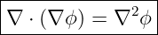
The next lesson, EM04, will combine spatial derivatives to introduce the Laplacian and the three-dimensional wave equation. In particular,

|----------------| |∇ ⋅ (∇ ϕ) = ∇2 ϕ| -----------------

(125)

will become the natural three-dimensional generalization of the second spatial derivative from the one-dimensional Wave mechanics series.

References

[1] H. M. Schey, Div, Grad, Curl, and All That, 4th ed., W. W. Norton & Company, 2005.

[2] David J. Griffiths, Introduction to Electrodynamics, 4th ed., Cambridge University Press, 2017.

[3] Gilbert Strang and Edwin “Jed” Herman, Calculus, Volume 3, OpenStax, 2016, chapters on vector fields and vector calculus.

[4] Massachusetts Institute of Technology, 18.02SC Multivariable Calculus, MIT OpenCourseWare, materials on gradient, divergence, curl, flux, and line integrals.

[5] Samuel J. Ling, Jeff Sanny, and William Moebs, University Physics, Volume 2, OpenStax, 2016, chapters on electric and magnetic fields and electromagnetic waves.

[6] Richard P. Feynman, Robert B. Leighton, and Matthew Sands, The Feynman Lectures on Physics, Volume II, Addison-Wesley, 1964, chapters on vector electromagnetic fields and Maxwell’s equations.

"Antennas Electromagnetic Waves" is owned by bloftin.
(view preamble)