Electromagnetic Waves, Antennas, and RF: From a 1D Wave to a Field
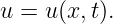
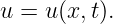
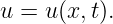
The wave mechanics series developed waves gradually from an oscillation at one point to quantities
that depend on both position and time. A typical one-dimensional wave was written
as
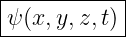
That notation already contains the central idea needed to begin Electromagnetism: a physical
quantity can be assigned to every point in space and can change with time. Such a quantity is
called a field.
Electromagnetism uses fields as its basic language. Electric and magnetic fields are not merely
single numbers attached to one object. They are quantities defined throughout space, and they can
vary from place to place and from instant to instant [1, 2, 3, 4].
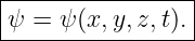
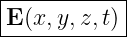
EM01 makes the transition in four small steps:
The first three expressions are scalar-valued. The last is vector-valued. Maxwell’s equations are
intentionally deferred. The goal here is only to become comfortable with what a field is and how
wave language extends from one spatial dimension to three.
1 A one-dimensional wave is already a field
Consider a one-dimensional wave
At a fixed time t = t0, the function becomes
Every position x is assigned one number u. That is already a scalar field on a one-dimensional
space.
For example, the snapshot
assigns a displacement to every point along the x axis.
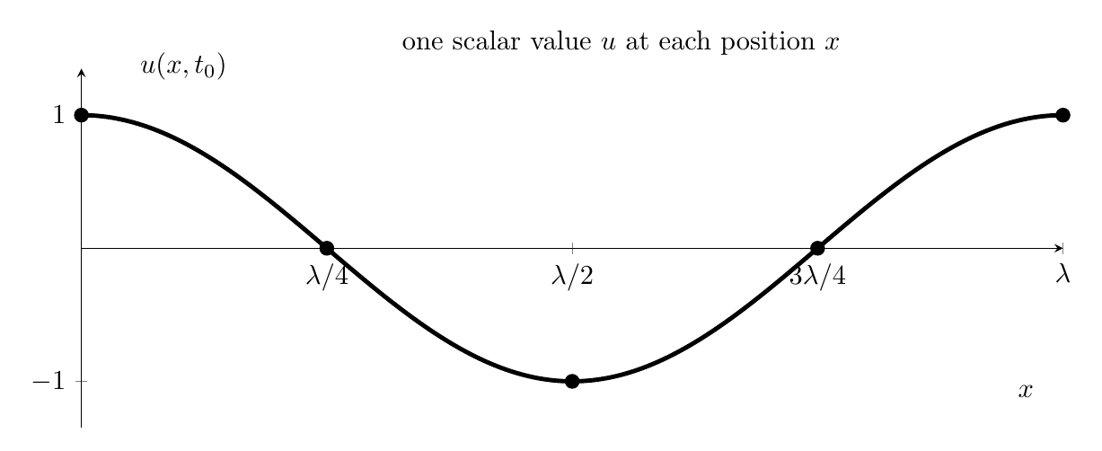
Figure. At one instant, a one-dimensional wave assigns one scalar value to every position
on the line. The plotted curve is therefore a picture of a scalar field in one spatial
dimension.
This viewpoint is more general than a vibrating string. The quantity u could represent pressure
perturbation, voltage, density perturbation, temperature variation, or another scalar-valued
physical quantity.
The essential structure is
2 Function notation as a map
It is useful to read
as an instruction:
Give the function a position x and a time t; the function returns the value of the
field there and then.
For example, if
then the number
is the value of the field at one particular event in space and time.
An event in this elementary sense is simply a specified place and time.
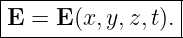
This language will be important later because electromagnetic fields such as
are evaluated in exactly the same way.
3 From one spatial coordinate to three
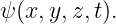
The simplest wave model uses one spatial coordinate:
A field in ordinary three-dimensional space can depend on
as well as time. A scalar field may therefore be written
At every point (x,y,z) and time t, the field returns one scalar number.
Examples of scalar fields include temperature,
and pressure,
The physical meaning differs, but the mathematics has the same structure.
4 A scalar-field snapshot
At a fixed time t = t0, a three-dimensional scalar field becomes
If we further examine only a plane such as z = 0, then
This can be drawn using contours. Each contour joins points with equal field value.
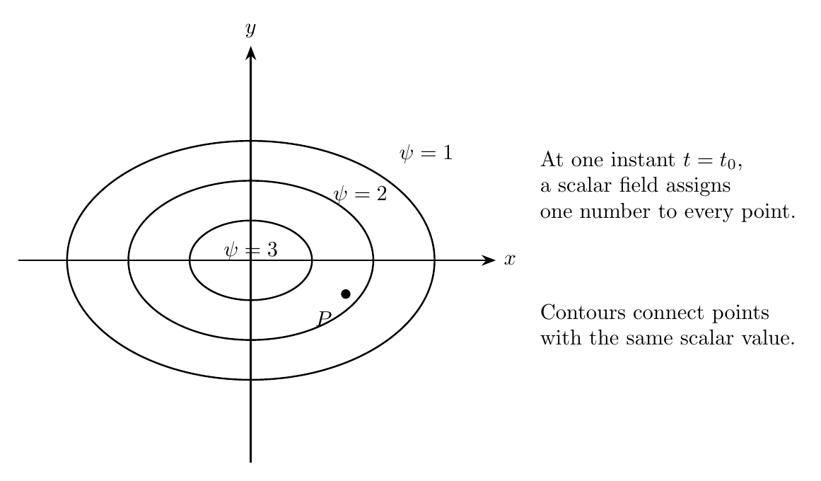
Figure. A two-dimensional slice through a scalar field at one instant. Each spatial point
has one scalar value, and a contour connects locations with the same value.
A contour plot is therefore not a trajectory of a moving particle. It is a map of field values across
space.
That distinction will matter later when electric-field lines and wavefronts are introduced. A line
drawn in a field diagram does not automatically mean that matter or energy physically travels
along that line.
5 The position vector
Writing all three coordinates repeatedly becomes cumbersome. We therefore introduce the position
vector
The notation
is shorthand for
Likewise,
means a vector field evaluated at position r and time t.
No new physics has been introduced by this notation. It is only a compact way to refer to a
location in three-dimensional space.
6 Scalar fields and vector fields
A scalar field assigns one number to every point. A vector field assigns a vector to every
point.
A two-dimensional vector field can be written
A three-dimensional vector field has three components:
Each component is itself a scalar field.
Thus a vector field can be understood as several scalar component fields combined with basis
directions.
7 The electric field is vector-valued
The Electric Field will eventually be defined physically through the force experienced by charge.
For now, we need only its mathematical type:
At each position and time, the electric field has both magnitude and direction.
In Cartesian coordinates,
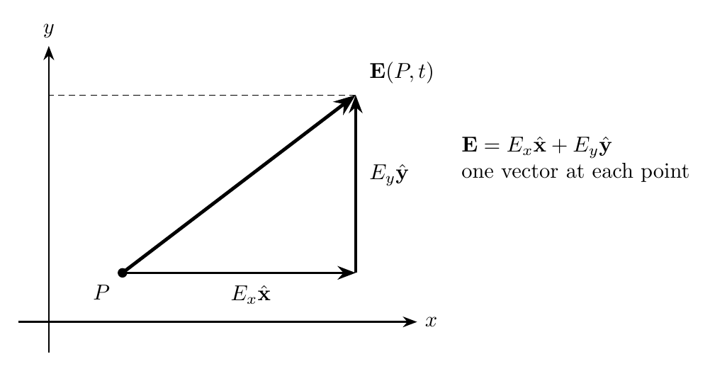
Figure. A vector field assigns a vector to each point. The vector can be decomposed into
Cartesian components such as Exx and Eyy.
EM02 will develop vector components, dot products, cross products, and transverse directions
more systematically.
8 A vector field is not a moving arrow
A common conceptual mistake is to imagine that the arrow representing a vector field is itself an
object moving through space.
Instead, at one instant the field specifies a vector at every position.
For example, suppose
At the point
we obtain
At another location, the vector can be different.
The collection of all these vectors is the field.
9 Two complementary ways to inspect a time-dependent field
A field that depends on space and time can be inspected in two especially useful ways.
9.1 Snapshot in space
Fix the time:
Then examine
This answers:
What does the field look like everywhere in space at this instant?
This is analogous to taking a photograph of a wave.
9.2 Time history at one point
Instead fix the position:
Then examine
This answers:
What does one detector at one location observe as time passes?
A radio receiver and a GPS antenna are physically much closer to this second viewpoint: the
hardware occupies a limited region of space and measures time-varying electromagnetic quantities
there.
10 The one-dimensional traveling-wave pattern survives
The Wave Mechanics series used expressions such as
The same mathematical idea survives in electromagnetism, but the field itself becomes
vector-valued.
A simple illustrative field is
Read this equation carefully:
- the field varies with z and t;
- the field vector points in the x direction;
- the pattern propagates in the +z direction because the phase is kz − ωt;
- the field direction and propagation direction are different.
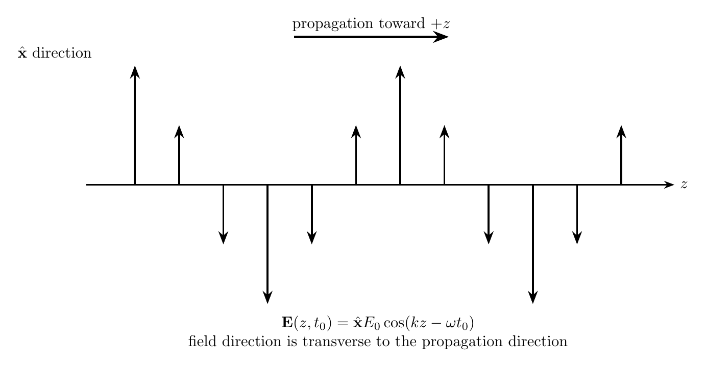
Figure. An illustrative transverse vector wave. The electric-field vector points along x
while the sinusoidal pattern propagates along +z.
The fact that electromagnetic waves are transverse will later follow from Maxwell’s equations.
EM01 uses the form only to show how a familiar one-dimensional sinusoid can become a vector
field.
11 Field direction versus direction of variation
The equation
contains two different directions.
The basis vector
tells us the direction in which the field vector points.
The coordinate
tells us the direction along which the phase changes in this example.
Confusing these two directions is a common early mistake.
A field can point in one direction while changing from place to place in another direction.
12 Field magnitude
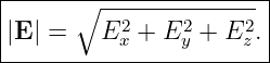
For a vector
its magnitude is
This is simply the three-dimensional Pythagorean theorem.
For the illustrative plane-wave field
we have
and
Therefore
The vector itself can point in either the positive or negative x direction as the sinusoid changes
sign.
13 A field may be uniform or nonuniform
A uniform vector field has the same vector at every spatial point. For example,
is spatially uniform at time t0.
By contrast,
is nonuniform because its value changes with z.
The words uniform and constant therefore need context. A field may be spatially uniform yet
change with time, or spatially varying yet frozen at one selected instant.
14 Fields and measurements
Fields are mathematical models, but they are tied to measurement.
A sensor located at r0 samples a field locally. If the field is
then the sensor encounters
That is a time history at one location.
Later, an antenna will be treated more carefully because a real antenna occupies a finite region and
responds to spatial structure, polarization, orientation, and phase across an aperture or array. But
the local-field viewpoint is the correct first step.
15 Why this matters for radio and GPS
A radio wave is not merely a scalar sinusoid moving through empty space. It is an electromagnetic
field distributed through space and time.
A GPS receiving antenna does not directly observe “the satellite power” as a single abstract
number. The satellite generates electromagnetic fields that propagate across a very large distance.
The receiving antenna interacts with the local electric and magnetic fields that arrive at its
aperture.
The later chain will be
Only after that chain is understood will quantities such as
and
be physically transparent rather than merely memorized link-budget formulas.
16 Worked Example 1: identify the type of field
Classify each expression as scalar or vector-valued.
| T(x,y,z,t) | = T0 + ax, | (51)
|
| p(x,t) | = p0 cos(kx − ωt), | (52)
|
| E(x,t) | = yE0 cos(kx − ωt). | (53) |
The first expression returns one temperature value at each event, so it is a scalar field.
The second returns one pressure value at each event, so it is also a scalar field.
The third returns a vector because the scalar coefficient multiplies a basis direction y. It is
therefore a vector field.
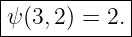
17 Worked Example 2: evaluate a scalar field
Suppose
Find the field at
Substitution gives
| ψ(3, 2) | = 2(3) − (2)2 | (56)
|
| = 6 − 4 | (57)
|
| = 2. | (58) |
Thus
The result is a scalar because the field itself is scalar-valued.
18 Worked Example 3: evaluate a vector field
Let
At
we obtain
Its magnitude is
| |E| | =  | (63)
|
| =  | (64)
|
| ≈ 6.32. | (65) |
Thus the vector field specifies both a direction and a magnitude at that point.
19 Worked Example 4: snapshot versus time history
Consider
A spatial snapshot at t = 0 is
A time history at the position x = 0 is
Since cosine is even,
These are two views of the same field: one shows variation across space at one time, and the other
shows variation in time at one position.
20 Worked Example 5: read a simple vector wave
Consider
Identify the field direction and propagation direction.
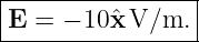
The basis vector x shows that the electric field points along the x axis.
The phase
has the same right-moving form studied in the Wave Mechanics series, so the pattern propagates
toward increasing z.
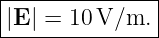
Therefore
and
The field is transverse in this illustrative example because the field direction is perpendicular to
the propagation direction.
21 Worked Example 6: evaluate the vector wave at one event
Using
suppose
and the phase at a particular event is
Then
so
The negative sign does not mean the field magnitude is negative. It means the vector points in the
−x direction at that event. Its magnitude is
22 Common mistakes
- Mistake: thinking a field is a single number for the whole system. A field assigns
values throughout space and time.
- Mistake: confusing a scalar field with a vector field. A scalar has magnitude only; a
vector has magnitude and direction.
- Mistake: interpreting a field arrow as a material object moving through space. The
arrow represents the field value at a location.
- Mistake: confusing the direction in which a vector points with the direction in which
its value changes spatially.
- Mistake: treating a contour as a path followed by the field. A contour simply joins
points of equal scalar value.
- Mistake: assuming that writing E(r,t) introduces new physics. It is compact notation
for a vector field depending on spatial coordinates and time.
23 What EM01 adds to the Wave Mechanics foundation
The Wave Mechanics series established the idea of a quantity such as
varying through one spatial coordinate and time.
EM01 generalizes that idea to
for a scalar field and
for a vector field.
The essential conceptual bridge is
No Maxwell equation is needed yet. EM02 next develops the vector mathematics needed to
describe electromagnetic fields cleanly: components, basis directions, dot products, cross products,
and the geometry of transverse fields.
References
[1] David J. Griffiths, Introduction to Electrodynamics, 4th ed., Cambridge University
Press, 2017.
[2] Samuel J. Ling, Jeff Sanny, and William Moebs, University Physics, Volume 2,
OpenStax, 2016, chapters on electric fields, magnetic fields, and electromagnetic waves.
[3] Richard P. Feynman, Robert B. Leighton, and Matthew Sands, The Feynman Lectures
on Physics, Volume II, Addison-Wesley, 1964, chapters introducing electromagnetic
fields.
[4] Massachusetts Institute of Technology, 8.02 Physics II: Electricity and Magnetism,
MIT OpenCourseWare, materials on electric and magnetic fields.
[5] Frank S. Crawford, Jr., Waves, Berkeley Physics Course, Volume 3, McGraw-Hill,
1968.