|
|
|
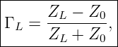
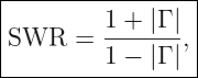
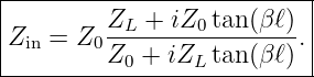
|||||||
and, for a lossless line of length ℓ,
These formulas are consequences of distributed electromagnetic wave propagation, not independent circuit rules [1, 2, 3, 4].
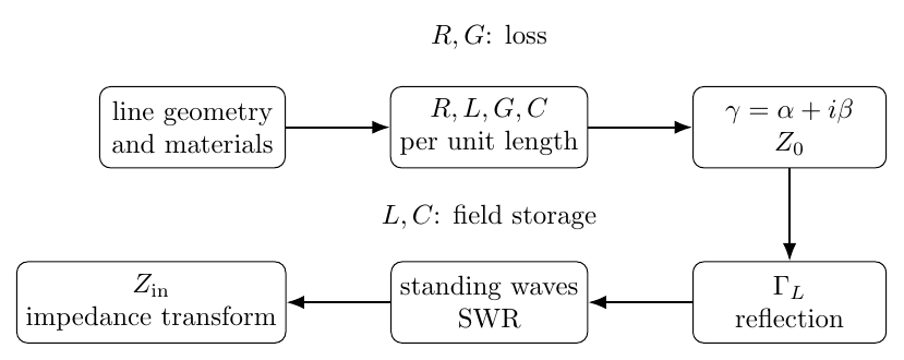
Figure. The calculation chain used throughout this problem set: physical line parameters lead to R,L,G,C, then to γ and Z0, and finally to reflection, standing waves, and transformed impedance.
Part I: Exercises
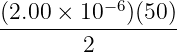
Exercise 1: recover the per-unit-length RLCG parametersA 2.00 m section of uniform transmission line has total series resistance 0.400 Ω, total series inductance 0.500 μH, total shunt conductance 4.00 μS, and total shunt capacitance 200 pF. Find R, L, G, and C per unit length. State the SI units of each quantity and identify which parameters represent stored field energy and which represent dissipation.
Exercise 2: exact propagation constant and characteristic impedanceAt f = 100 MHz, a uniform line has
Using the exact formulas, calculate
Exercise 3: test the low-loss approximationFor the line in Exercise 2:
Exercise 4: an ideal lossless lineA lossless line has
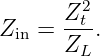
Find
Exercise 5: complex load reflection coefficientA lossless 50 Ω line is terminated by
Calculate the load reflection coefficient ΓL in rectangular and polar form. Interpret the magnitude and phase physically.
Exercise 6: reflected power, return loss, and SWRContinue Exercise 5. Find
If the forward voltage-wave phasor amplitude is |V +| = 10 V, calculate the forward, reflected, and net average powers.
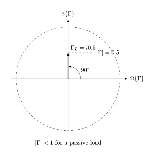
Figure. The complex reflection coefficient contains two different pieces of information: |Γ| controls reflected-wave magnitude and SWR, while arg Γ controls where the standing-wave pattern sits relative to the load.
Exercise 7: standing-wave maxima and minimaA lossless line has wavelength
and load reflection coefficient
Let d ≥ 0 denote distance measured from the load back toward the generator. If |V +| = 4.00 V, determine
Exercise 8: infer mismatch magnitude and phase from an SWR measurementA lossless line has wavelength 24.0 cm. A slotted-line measurement gives
and the nearest voltage maximum is 3.00 cm from the load toward the generator. Determine |ΓL| and one equivalent value of arg ΓL in the interval (−180∘, 180∘].
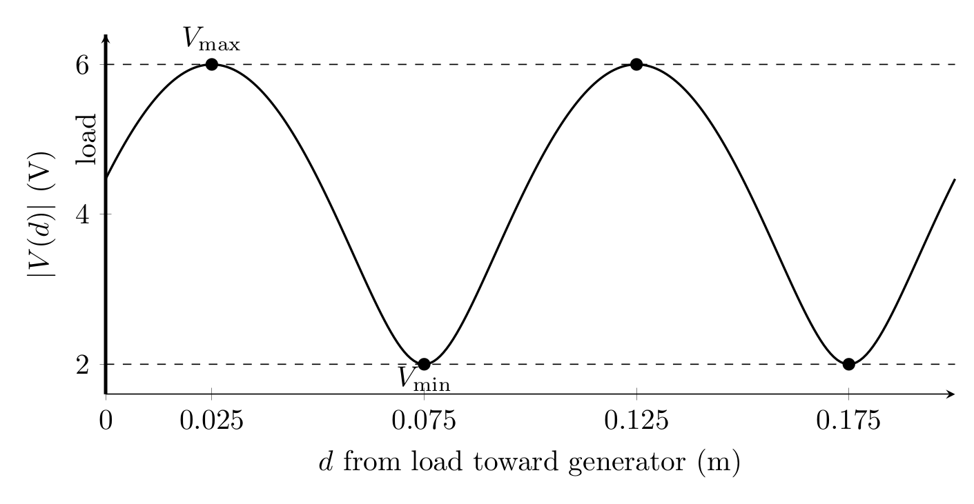
Figure. For a lossless line, the phase of ΓL shifts the standing-wave pattern. Magnitude controls the envelope contrast; phase controls the positions of maxima and minima.
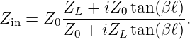
Exercise 9: input impedance of a finite lossless lineA 50 Ω lossless line is terminated in
The line length is
Find the input impedance Zin.
Exercise 10: quarter-wave impedance transformerA 50 Ω feed line must be matched to a purely resistive 100 Ω load at one design frequency using a lossless quarter-wave transformer. Find the required characteristic impedance Zt of the transformer section and verify algebraically that the input impedance looking into the quarter-wave section is 50 Ω.
Exercise 11: short-circuited lineA lossless 50 Ω line is terminated in a short circuit. Derive
Then evaluate the input impedance for
Interpret each result.
Exercise 12: open-circuited lineA lossless 50 Ω line is terminated in an open circuit. Derive
Evaluate the same three lengths λ∕8, λ∕4, and λ∕2. Compare the results with the short-circuit case.
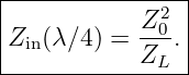
Exercise 13: the quarter-wave impedance inverterStarting from the lossless input-impedance formula, prove that a quarter-wave section obeys
Use this to explain why a quarter-wave line transforms an open circuit into a short circuit and a short circuit into an open circuit.
Exercise 14: coaxial-line geometry to C, L, Z0, and velocityA lossless coaxial cable has inner-conductor radius
outer-conductor inner radius
and a homogeneous dielectric with
Use
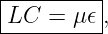
to calculate C, L, Z0, and vp. Verify explicitly that LC = μ𝜖.
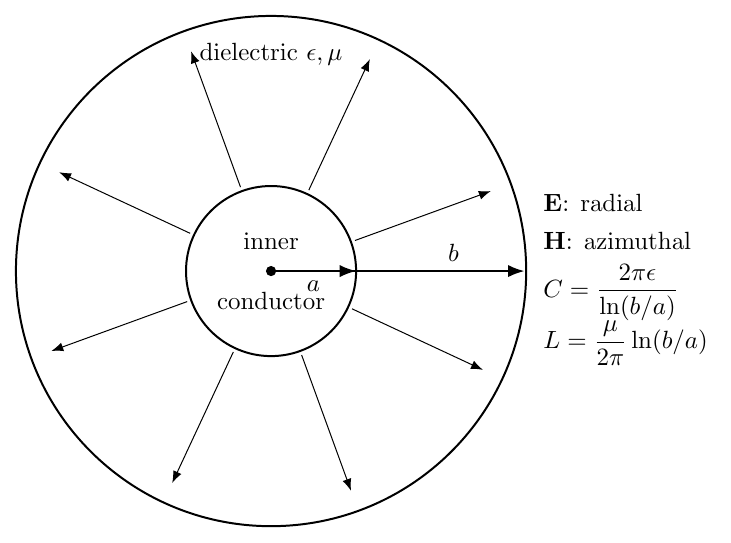
Figure. Coaxial geometry converts the full transverse electromagnetic field problem into per-unit-length L and C. Their product fixes wave speed; their ratio fixes characteristic impedance.
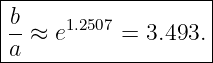
Exercise 15: design the coax radius ratio for 50 ΩFor a lossless nonmagnetic coax filled with 𝜖r = 2.25, choose the radius ratio b∕a required for
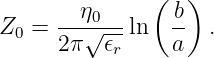
Use
If a = 0.500 mm, determine b.
Exercise 16: Julia sweep of load impedance and line lengthWrite a Julia program for a lossless 50 Ω line that:
Part II: Complete Worked Solutions
Solution 1: recover the per-unit-length RLCG parametersFor a uniform line, each distributed parameter equals the total value divided by the physical length. For resistance,
For inductance,
For conductance,
For capacitance,
The parameters L and C represent magnetic and electric field-energy storage. The parameters R and G represent Conductor and dielectric dissipation. The dimensions are therefore
Solution 2: exact propagation constant and characteristic impedanceThe angular frequency is
The series impedance per unit length is
The shunt admittance per unit length is
Therefore
Evaluating the complex square root gives
Thus
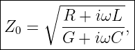
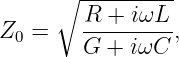
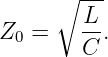
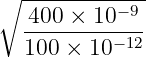
The characteristic impedance is
which gives
Its polar form is
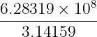
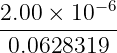
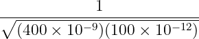
The wavelength is
Finally,
The line is very nearly lossless in phase and impedance, but the exact solution retains a small attenuation and a tiny impedance phase angle.
Solution 3: test the low-loss approximationFirst,
and
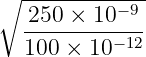
Both ratios are much less than one, so the low-loss approximation is strongly justified. The lossless characteristic impedance is
Then
Also,
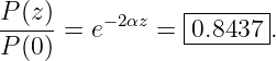
These agree with the exact result to the displayed precision. After z = 100 m, a forward voltage amplitude is multiplied by
Power is quadratic in amplitude, so
The power loss in decibels is
Equivalently, the positive insertion loss magnitude is 0.738 dB.
Solution 4: an ideal lossless lineFor a lossless line,
Therefore
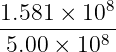
The propagation speed is
At f = 500 MHz,
Then
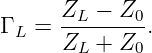
Solution 5: complex load reflection coefficientUse
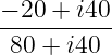
Substituting ZL = 30 + i40 Ω and Z0 = 50 Ω,
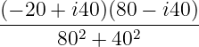
Multiply numerator and denominator by 80 − i40:
Thus
The magnitude says that the reflected voltage-wave amplitude is half the incident amplitude. The phase says that the reflected voltage at the load leads the incident voltage by 90∘.
Solution 6: reflected power, return loss, and SWRBecause reflected power is proportional to squared voltage amplitude,
For a lossless line and passive load, the delivered fraction is
The SWR is
The return loss is
With |V +| = 10 V and real Z 0 = 50 Ω,
The reflected wave has |V −| = |Γ||V +| = 5 V, so
Hence
Solution 7: standing-wave maxima and minimaFor a lossless line measured by distance d = −z from the load toward the generator,
Here
The envelope extrema are
A maximum occurs when
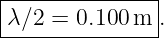
For the nearest nonnegative distance, choose m = 0:
A minimum occurs when
The nearest positive solution uses m = −1:
Adjacent maxima are separated by
Solution 8: infer mismatch magnitude and phase from an SWR measurementInvert the SWR relation:
For a voltage maximum at distance d from the load,
For the nearest maximum and the principal phase, use m = 0:
Therefore
SWR alone gives only the magnitude. A spatial reference such as a measured maximum location is needed to recover the phase.
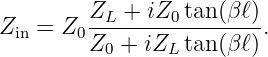
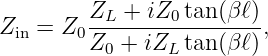
Solution 9: input impedance of a finite lossless lineUse
Since
we have
Therefore
Carrying out the complex division gives
The load itself has not changed; the line has transformed the voltage-current ratio observed at the input plane.
Solution 10: quarter-wave impedance transformerFor a lossless quarter-wave section,
To make this equal to the 50 Ω feed impedance,
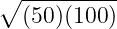
Thus
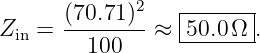
Verification is immediate:
The transformer is narrowband because the quarter-wave condition is tied to frequency through βℓ = π∕2.
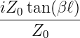
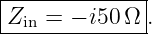
Solution 11: short-circuited lineSet ZL = 0 in the lossless input-impedance equation:
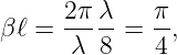
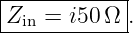
For ℓ = λ∕8,
so
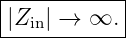
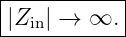
The input appears purely inductive. For ℓ = λ∕4,
and tan(π∕2) diverges, so ideally
The short has been transformed into an open. For ℓ = λ∕2,
so
The original short repeats after one half wavelength.
Solution 12: open-circuited lineTake the limit ZL →∞ in
Divide numerator and denominator by ZL and take the limit:
Thus
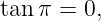
For ℓ = λ∕8,
so
The input appears purely capacitive. For ℓ = λ∕4,
so
The open becomes a short. For ℓ = λ∕2, cot π diverges, so
The original open repeats.
Solution 13: the quarter-wave impedance inverterFor
we have
Starting from
let T = tan(βℓ) and take the limit |T|→∞:
Therefore, if ZL →∞,
and if ZL → 0,
The quarter-wave section is therefore an impedance inverter.
Solution 14: coaxial-line geometry to C, L, Z0, and velocityThe material parameters are
With 𝜖r = 2.25 and μr = 1,
The radius ratio is
so
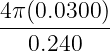
Therefore
and
Then
The wave speed is
Finally,
while
Thus
which is the transmission-line form of the electromagnetic wave-speed relation.
Solution 15: design the coax radius ratio for 50 ΩFor a nonmagnetic dielectric,
Therefore
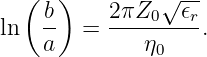
Solve for the ratio:
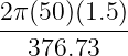
Using η0 ≈ 376.73 Ω,
Hence
For a = 0.500 mm,
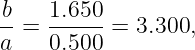
The required impedance depends on the radius ratio, not on the absolute scale, so scaling both radii by the same factor leaves ideal Z0 unchanged.
Solution 16: Julia sweep of load impedance and line lengthOne implementation is:
using Printf

Z0 = 50.0

println("Resistive-load sweep")
for ZL in range(10.0, 200.0, length=20)
    Gamma = (ZL - Z0) / (ZL + Z0)
    Rpow = abs2(Gamma)
    swr = (1 + abs(Gamma)) / (1 - abs(Gamma))
    @printf("ZL=%7.2f ohm  Gamma=% .5f  R=%7.5f  SWR=%7.4f\n",
            ZL, Gamma, Rpow, swr)
end

ZL = 30.0 + 40.0im
println("\nLength sweep for ZL = 30 + j40 ohm")
for ell_over_lambda in range(0.0, 0.5, length=21)
    theta = 2*pi*ell_over_lambda
    # Avoid the tan singularity exactly at lambda/4 by using the
    # reflection-coefficient form when desired; ordinary complex
    # arithmetic is sufficient away from the exact singular point.
    if abs(cos(theta)) > 1e-10
        t = tan(theta)
        Zin = Z0 * (ZL + 1im*Z0*t) / (Z0 + 1im*ZL*t)
        @printf("ell/lambda=%6.3f  Zin=%9.3f %+.3fj ohm\n",
                ell_over_lambda, real(Zin), imag(Zin))
    end
end

GammaL = (ZL - Z0) / (ZL + Z0)

# Stable all-length form using Gamma at the observation plane:
function zin_from_gamma(Z0, GammaL, ell_over_lambda)
    Gamma_in = GammaL * exp(-1im*4*pi*ell_over_lambda)
    return Z0 * (1 + Gamma_in) / (1 - Gamma_in)
end

Zhalf = zin_from_gamma(Z0, GammaL, 0.5)
Zquarter = zin_from_gamma(Z0, GammaL, 0.25)


@printf("\nZin at lambda/2 = %.6f %+.6fj ohm\n",
        real(Zhalf), imag(Zhalf))
@printf("expected ZL     = %.6f %+.6fj ohm\n",
        real(ZL), imag(ZL))
@printf("Zin at lambda/4 = %.6f %+.6fj ohm\n",
        real(Zquarter), imag(Zquarter))
@printf("Z0^2/ZL         = %.6f %+.6fj ohm\n",
        real(Z0^2/ZL), imag(Z0^2/ZL))
For the fixed complex load,
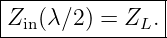
At a half wavelength,
so the input reflection coefficient equals the load reflection coefficient and
At a quarter wavelength,
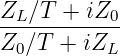
and the input impedance becomes
The numerical sweep therefore checks both periodicity and quarter-wave inversion without relying only on symbolic algebra.
What EM22E1 adds to the seriesEM22 derived the distributed-wave model. EM22E1 makes that model operational. The worked problems connect physical line geometry to R,L,G,C, then to
The key conceptual point is that transmission-line effects are not corrections to ordinary lumped circuits. They are wave phenomena. Once line dimensions and timing make propagation delay important, voltage and current must be treated as traveling fields with phase, attenuation, reflection, and interference. This prepares the series for radiation from time-varying currents, where guided electromagnetic energy leaves the transmission structure and becomes a freely propagating antenna field.
References
References
[1] David M. Pozar, Microwave Engineering, 4th ed., Wiley, 2012. [2] Robert E. Collin, Foundations for Microwave Engineering, 2nd ed., Wiley-IEEE Press, 2001. [3] Simon Ramo, John R. Whinnery, and Theodore Van Duzer, Fields and Waves in Communication Electronics, 3rd ed., Wiley, 1994. [4] Fawwaz T. Ulaby and Umberto Ravaioli, Fundamentals of Applied Electromagnetics, 7th ed., Pearson, 2015. [5] Matthew N. O. Sadiku, Elements of Electromagnetics, 7th ed., Oxford University Press, 2018. "Electromagnetic Waves, Antennas, and RF: Transmission Lines - Exercises and Complete Worked Solutions" is owned by bloftin.
This object's parent. Cross-references: energy, radiation, wave phenomena, speed, square, shunt admittance per unit length, series impedance per unit length, dimensions, Conductor, program, input impedance, generator, average powers, SWR, magnitude, load reflection coefficient, phase constant, power, velocity, field energy, unit, capacitance, conductance, inductance, resistance, transmission line, section, electromagnetic wave, formulas, relations, impedance, Standing Waves, characteristic impedance, propagation constant, parameters, telegrapher's equations, EM22 This is version 1 of Electromagnetic Waves, Antennas, and RF: Transmission Lines - Exercises and Complete Worked Solutions, born on 2026-10-09. Object id is 1448, canonical name is ElectromagneticWavesAntennasAndRFTransmissionLinesExercisesAndCompleteWorkedSolutions. Accessed 8 times total. Classification:
|
|
|
|
Pending Errata and AddendaNone.
|
DiscussionNo messages.
|
Interact |
![[parent]](https://images.physicslibrary.org/images/uparrow.png)




 ;
;


















![[R ] = Ω∕m, [L ] = H/m, [G] = S/m, [C ] = F/m.](https://images.physicslibrary.org/cache/objects/1448/make4ht/ElectromagneticWavesAntennasAndRFTransmissionLinesExercisesAndCompleteWorkedSolutions30x.png)











 +
+ 
 +
+ 











 = 0
= 0
![[ ]
|V(d)|2 = |V + |2 1 + |Γ |2 + 2|Γ |cos(ϕ − 2βd) .](https://images.physicslibrary.org/cache/objects/1448/make4ht/ElectromagneticWavesAntennasAndRFTransmissionLinesExercisesAndCompleteWorkedSolutions74x.png)


































 ln(
ln(