|
|
|
|||||||
and
For Love exterior equivalence, where the replacement field is zero on the interior side,
Three numerical ideas are used repeatedly in the problems. A far-field phase error is the difference between the exact propagation phase −kR and the phase obtained after replacing R by its far-field approximation. A discrete Huygens-source approximation replaces a continuous surface or line integral by a finite weighted sum. The resulting difference from the continuous-aperture result is the aperture sampling error.
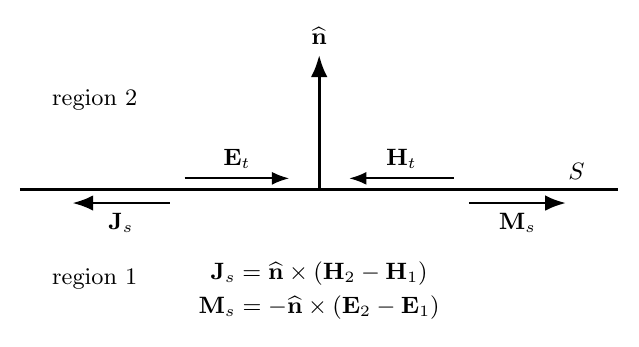
Figure 1. Region ordering, surface normal, and tangential fields determine the signs of the equivalent electric and magnetic surface currents.
Part I: Exercises
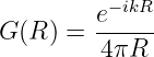
Exercise 1: outgoing Green-function phase and amplitudeAt f = 1.00 GHz in free space, compare the outgoing scalar Green function
at
Find the magnitude ratio |G(R2)∕G(R1)| and the phase change from R1 to R2.
Exercise 2: surface currents from general field jumpsA planar interface has
The tangential fields on the two sides are
Find Js and Ms.
Exercise 3: Love currents for a normally incident plane waveA free-space plane wave propagates in the +z direction with
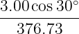
Take the Huygens surface at z = 0 with n = z. Find the Love-equivalent Js and Ms that reproduce the exterior wave and give zero interior field. Use η0 = 376.73 Ω.
Exercise 4: reversing the chosen surface normalRepeat Exercise 3 with the geometric surface normal reversed:
Using the corresponding Love formulas with n′, determine how the signed equivalent currents change.
Exercise 5: complementary interior-field equivalenceLet region 1 be the interior of a closed surface and region 2 the exterior, with n pointing outward. Construct a replacement problem that preserves the original fields E,H in region 1 but forces the replacement fields to zero in region 2. Derive the required Js and Ms.
Exercise 6: oblique TE plane wave on a Huygens planeA free-space plane wave propagates in the x-z plane at
from the +z axis. Its electric field is TE-polarized,
with
For the plane z = 0 with n = z, find H, Js, and Ms.
Exercise 7: complex polarization and equivalent currentsAt z = 0, a normally propagating +z free-space wave has phasor electric field
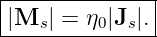
Find H, Js, and Ms for n = z. Verify the magnitude relation between Ms and Js.
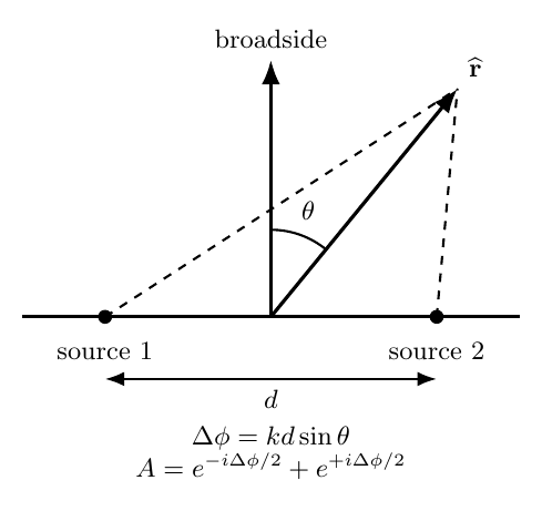
Exercise 8: two discrete Huygens sourcesTwo equal in-phase elementary Huygens sources are separated by
along the x axis. In the x-z plane, the far-field phase difference is
Ignoring the common element pattern, find the magnitude of the coherent sum at 𝜃 = 0∘, 30∘, and 90∘, normalized so that one source alone has amplitude 1.
Figure 2. Two separated Huygens sources acquire an observation-angle-dependent path difference. Their complex fields must be added before magnitudes or powers are formed.
Exercise 9: quantify a far-field phase approximationFor an aperture point at
an observation distance
and observation angle
use
and
Find the path-length error, the associated phase error in degrees, and the ratio between the exact 1∕R amplitude factor and the common far-field factor 1∕r.
Exercise 10: discrete Huygens approximation to a continuous apertureA uniform line aperture has width
Its normalized continuous aperture factor is
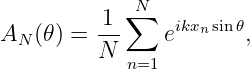
Approximate the aperture by N equally weighted midpoint Huygens sources,
where the xn are the subinterval midpoints. At 𝜃 = 10∘, evaluate |A| and |A N| for N = 4, 8, 16, 32. Report the percentage magnitude error.
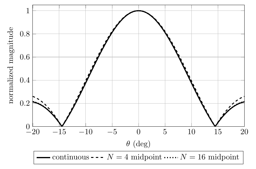
Figure 3. Midpoint Huygens-source sampling converges toward the continuous uniform-aperture pattern as the number of source samples increases.
Exercise 11: first null of a uniform apertureA uniformly illuminated one-dimensional aperture has width
Find the first null angle measured from broadside.
Exercise 12: half-power beamwidth of the 4λ apertureFor a uniform aperture with
solve numerically for the positive angle 𝜃hp at which
Find the full half-power beamwidth
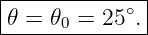
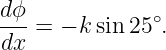
Exercise 13: steering a continuous aperture with a phase rampA uniform line aperture of width D = 4λ is given the excitation phase
with
Show where the main beam points. Find the phase slope dϕ∕dx in rad/λ, the total phase change from x = −D∕2 to x = +D∕2, and the phase step between samples spaced by d = λ∕2.
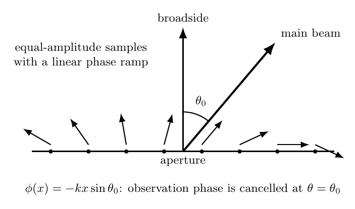
Figure 4. A linear phase ramp across an aperture cancels the observation phase in one selected direction and therefore steers the main beam.
Exercise 14: conducting-screen aperture equivalenceAn aperture in a large conducting screen has tangential electric field
With n = z directed into the radiating half-space, use the common aperture-equivalence convention
Find Ms and state its units.
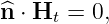
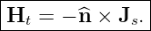
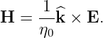
Exercise 15: recover tangential fields from Love currentsFor Love exterior equivalence with outward normal n, suppose the equivalent currents are known. Starting from
derive formulas for the tangential fields Et and Ht in terms of Js and Ms.
Exercise 16: synthesis check from surface fields to a sampled aperture patternA 4λ uniform aperture is represented by N = 16 equally spaced midpoint Huygens samples. At 𝜃 = 10∘, compare the sampled magnitude |A 16| with the exact continuous magnitude |A|. Then state what would happen to the sampled pattern if every equivalent current sample were multiplied by the same complex constant Ceiϕ0.
Part II: Complete Worked Solutions
Solution 1: outgoing Green-function phase and amplitudeThe free-space wavelength is
Hence
The magnitude of the Green function is 1∕(4πR), so
The unwrapped phase change is
Modulo 360∘, this is equivalent to
Thus increasing range reduces amplitude by the geometric 1∕R factor and advances the negative outgoing-wave phase by 300.21∘.
Solution 2: surface currents from general field jumpsFirst form the field jumps:
Using
we obtain
and
Therefore
Solution 3: Love currents for a normally incident plane waveFor a +z free-space plane wave,
Numerically,
Then
Hence
Solution 4: reversing the chosen surface normalWith
the same algebraic Love formulas give
and
Therefore
Equivalent-current signs are orientation dependent. A surface normal must always be stated together with the current convention.
Solution 5: complementary interior-field equivalenceFor the desired replacement problem,
in the interior, while
in the exterior. The jump conditions give
Thus
The signs are the reverse of the usual Love exterior-equivalence currents because the prescribed field jump has been reversed.
Solution 6: oblique TE plane wave on a Huygens planeFor a plane wave,
Using
and E = E0y,
Hence
The Love electric surface current is
The equivalent magnetic surface current is
Therefore
Only the tangential part of H contributes to Js on the z = 0 surface.
Solution 7: complex polarization and equivalent currentsFor propagation along +z,
Then
and
The electric-field magnitude is
Therefore
so
The result holds for normal-incidence free-space plane waves even when the polarization state is complex.
Solution 8: two discrete Huygens sourcesWith d = λ∕2,
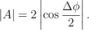
Two equal phasors separated symmetrically in phase have total magnitude
At broadside,
At 30∘,
At endfire,
Thus
Solution 9: quantify a far-field phase approximationNormalize lengths by λ. With r = 100λ, x = 2λ, and sin 30∘ = 0.5,
whereas
The path error is
The phase error magnitude is
For amplitude,
Therefore
The approximation is already good in amplitude, while the phase error is the more sensitive quantity.
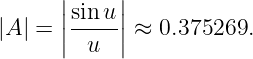
Solution 10: discrete Huygens approximation to a continuous apertureAt 𝜃 = 10∘ and D = 4λ,
Therefore
Using midpoint samples gives
Thus the discrete Huygens sum converges rapidly toward the continuous aperture integral:
The numerical trend also shows why a sampled array and a continuous aperture become closely related when the spatial sampling is sufficiently fine.
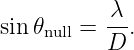
Solution 11: first null of a uniform apertureFor a uniform line aperture,
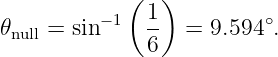
With D = 6λ,
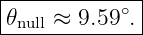
Therefore
Increasing aperture width narrows the main lobe.
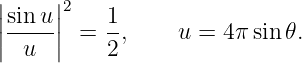
Solution 12: half-power beamwidth of the 4λ apertureThe half-power condition is
The positive root inside the main lobe is
The pattern is symmetric about broadside, so
Thus
Solution 13: steering a continuous aperture with a phase rampThe aperture integrand contains the product of the imposed excitation phase and the observation phase:
All aperture points are in phase when
For the main beam near broadside,
The phase slope is
Expressing x in wavelengths,
Across D = 4λ,
For d = λ∕2 sampling,
The phase ramp steers because it precompensates the free-space propagation phase in the selected direction.
Solution 14: conducting-screen aperture equivalenceUsing
with n = z and Ea = 4x V/m,
Therefore
Magnetic surface-current density has units V/m in this equivalence convention.
Solution 15: recover tangential fields from Love currentsStart with
Cross both sides with n:
Because Ht is tangential,
and the vector triple-product identity gives
Hence
Similarly,
Crossing with n gives
Therefore
This inversion is useful when a numerical or measured equivalent-current distribution is used as the surface data.
Solution 16: synthesis check from surface fields to a sampled aperture patternFrom Solution 10, the continuous 4λ aperture at 10∘ has
For N = 16 midpoint Huygens samples,
The magnitude difference is
corresponding to
relative magnitude error. Now multiply every equivalent source by the same complex constant Ceiϕ0. The whole discrete sum is multiplied by that same factor:
Therefore the normalized angular pattern is unchanged. The absolute field magnitude is scaled by |C|, the common phase is shifted by ϕ0, and the power scale changes by |C|2. Beam direction, null angles, and normalized sidelobe structure remain unchanged.
SummaryThe exercises demonstrate four central habits for equivalence-principle calculations:
EM30 can now use these skills to derive radiation from continuous apertures without treating the surface integral as a purely formal expression.
References
References
[1] A. E. H. Love, “The integration of the equations of propagation of electric waves,” Philosophical Transactions of the Royal Society of London A, vol. 197, pp. 1–45, 1901. [2] S. A. Schelkunoff, “Some equivalence theorems of electromagnetics and their application to radiation problems,” Bell System Technical Journal, vol. 15, no. 1, pp. 92–112, 1936. [3] R. F. Harrington, Time-Harmonic Electromagnetic Fields, IEEE Press, 2001 reissue of the 1961 text. [4] C. A. Balanis, Antenna Theory: Analysis and Design, 4th ed., Wiley, 2016. [5] W. L. Stutzman and G. A. Thiele, Antenna Theory and Design, 3rd ed., Wiley, 2012. "Electromagnetic Waves, Antennas, and RF: Huygens Principle and Electromagnetic Field Equivalence - Exercises" is owned by bloftin.
This object's parent. Cross-references: surface integral, radiation, cross products, identity, vector, algebraic, powers, electric field, forces, formulas, magnitude, function, scalar, line integral, relations, Normal, unit, Huygens surfaces, EM29 This is version 1 of Electromagnetic Waves, Antennas, and RF: Huygens Principle and Electromagnetic Field Equivalence - Exercises, born on 2026-10-10. Object id is 1465, canonical name is ElectromagneticWavesAntennasAndRFHuygensPrincipleAndElectromagneticFieldEquivalenceExercises. Accessed 2 times total. Classification:
|
|
|
|
Pending Errata and AddendaNone.
|
DiscussionNo messages.
|
Interact |
![[parent]](https://images.physicslibrary.org/images/uparrow.png)















































 (
( (2
(2
















![exp [− ikx sin 𝜃0]exp[ikx sin 𝜃] = exp[ikx(sin𝜃 − sin𝜃0)].](https://images.physicslibrary.org/cache/objects/1465/make4ht/ElectromagneticWavesAntennasAndRFHuygensPrincipleAndElectromagneticFieldEquivalenceExercises78x.png)