Complete CNAV Numerical Solution: IS-GPS-200 Table 30-II from Broadcast Parameters to ECEF State

1 Purpose and document status

GPSORB16 closed the legacy LNAV chain by evaluating Table 20-IV from one decoded ephemeris all the way to ECEF position, velocity, and acceleration. GPSORB17 then showed that CNAV retains the same geometric backbone but adds explicit secular freedom through ΔA, Ȧ, Δn₀, and Δṅ₀. The natural next step is to perform the complete CNAV calculation with one internally consistent set of numbers.

The computation developed here is

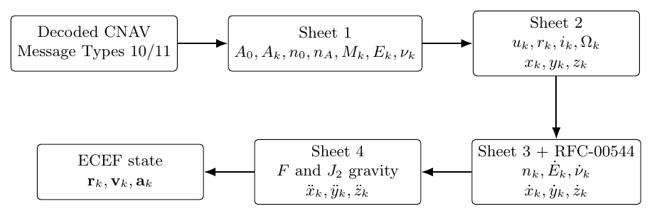
decoded CNAV ephemeris −→ rECEF −→ vECEF − → aECEF . k k k

(1)

Figure 1. End-to-end CNAV computation through Table 30-II.

The formally issued public baseline remains IS-GPS-200N together with its issued interface revision notices. In June 2026, the Public Interface Control Working Group accepted the substantive RFC-00544 material addressing the CNAV eccentric-anomaly-rate defect and related no-cost changes. The current issued-document index, however, lists IRN-004 as the RFC-00519 Civil ISM update rather than an incorporation of RFC-00544. Therefore this article uses the Revision-N Table 30-II position equations exactly as issued, and uses the accepted RFC-00544 corrected formulas for the CNAV velocity calculation. This distinction is important for both mathematical correctness and configuration control [1, 2, 3, 4].

2 Constants and worked-example parameters

Table 30-II uses the GPS user constants

μ = 3.986005 × 1014 m3∕s2,

(2)

˙Ωe = 7.2921151467 × 10−5 rad∕s,

(3)

and, for CNAV,

A = 26,559,710 m. REF

(4)

For the acceleration sheet,

RE = 6378137.0 m, J2 = 0.0010826262.

(5)

IS-GPS-200N specifies

π = 3.1415926535898

(6)

for the sensitive semicircle-to-radian conversion used in the broadcast user equations [1].

The example is synthetic, not an archived operational SV message. It is nevertheless placed on the Table 30-I broadcast quantization grid before conversion to computation units. That makes the numbers realistic enough for implementation testing while keeping the example reproducible.

parameter	Value used	Computation units
ΔA	290.000000	m
Semimajor-axis rate	1.49998665 × 10⁻²	m/s
Δn₀	4.50000887 × 10⁻⁹	rad/s
Mean-motion-difference rate	−3.00000289 × 10⁻¹³	rad/s²
M₀	0.9999999999	rad
e	0.01000000001	1
ω	0.7000000001	rad
t_oe	345600	s
t	352800	s
i₀	0.9599310884	rad
IDOT	−2.00008331 × 10⁻¹⁰	rad/s
Ω₀	1.1999999997	rad
Node-rate difference	1.68221293 × 10⁻¹⁰	rad/s

The harmonic coefficients are

Parameter	Value used	Units
C_us	8.00006092 × 10⁻⁶	rad
C_uc	1.00024045 × 10⁻⁶	rad
C_rs	80.000000	m
C_rc	200.000000	m
C_is	−2.00234354 × 10⁻⁷	rad
C_ic	9.96515155 × 10⁻⁸	rad

The CNAV node-rate reference is

Ω˙ = − 2.6 × 10−9 semicircles/s = − 8.1681408993 × 10−9 rad∕s. REF

(7)

Thus the fitted full node rate is

˙ ˙ ˙ −9 Ω = ΩREF + Δ Ω = − 7.9999196065 × 10 rad ∕s.

(8)

3 Sheet 1: semimajor axis, mean motion, and anomaly

Reference-time semimajor axis

CNAV does not broadcast the full semimajor axis directly. It broadcasts a difference from the fixed reference value:

A0 = AREF + ΔA.

(9)

For the example,

A0 = 26,560,000 m.

(10)

Time-varying semimajor axis

Table 30-II next gives

A = A + A˙t . k 0 k

(11)

The elapsed ephemeris time is

t = t − t = 352800 − 345600 = 7200 s, k oe

(12)

which requires no week-crossover correction. Therefore

Ak = 26,560,107.9990 m.

(13)

The secular size drift over two hours is approximately

Ak − A0 = 107.9990 m.

(14)

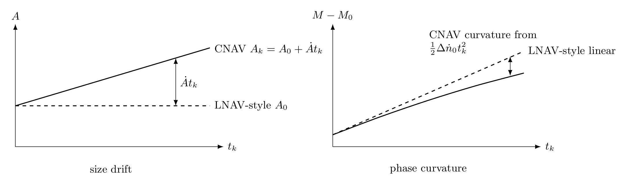
Figure 2. CNAV adds explicit semimajor-axis drift and mean-anomaly curvature relative to a matched LNAV-style propagation.

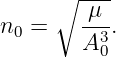
Computed reference mean motion

The Keplerian reference mean motion is computed from A₀, not the time-varying A_k:

∘ ---- n = μ--. 0 A30

(15)

Numerically,

−4 n0 = 1.45856844440235 × 10 rad∕s.

(16)

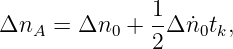
Revision-N interval-average mean-motion correction

The issued Table 30-II sheet 1 packages the correction as

1- ΔnA = Δn0 + 2Δ n˙0tk,

(17)

n = n + Δn . A 0 A

(18)

At two hours,

−9 ΔnA = 3.42000783094 × 10 rad ∕s,

(19)

− 4 nA = 1.45860264448066 × 10 rad∕s.

(20)

The important interpretation is that n_A is the interval-average corrected phase rate needed by the next line. It is not the instantaneous derivative of the mean anomaly when Δṅ₀≠0.

Mean anomaly

Table 30-II gives

Mk = M0 + nAtk.

(21)

Substituting the definition of n_A shows the underlying quadratic law:

( ) M = M + n + Δn + 1Δ ˙n t t . k 0 0 0 2 0 k k

(22)

Equivalently,

Mk = M0 + (n0 + Δn0 )tk + 1-Δ ˙n0t2. 2 k

(23)

For the example,

M = 2.05019390391426 rad. k

(24)

Newton solution of Kepler’s equation

Solve

Mk = Ek − esinEk

(25)

with

Ej = Ej− 1 + Mk-−-Ej-−1 +-esinEj-−1, E0 = Mk. 1 − ecos Ej−1

(26)

The iteration is

Iteration	E (rad)
0	2.050193903914264
1	2.059025896303176
2	2.059025552393593
3	2.059025552393593

Thus

Ek = 2.05902555239359 rad.

(27)

True anomaly

A quadrant-safe implementation uses

(√ ------ ) νk = atan2 1 − e2sinEk, cosEk − e .

(28)

This gives

ν = 2.06783669911589 rad. k

(29)

4 Sheet 2: corrected orbit geometry and ECEF position

The argument of latitude before periodic correction is

Φk = νk + ω = 2.76783669925706 rad.

(30)

The second-harmonic corrections are

δu_k	= C_us sin 2Φ_k + C_uc cos 2Φ_k,	(31)
δr_k	= C_rs sin 2Φ_k + C_rc cos 2Φ_k,	(32)
δi_k	= C_is sin 2Φ_k + C_ic cos 2Φ_k.	(33)

Numerically,

−6 δuk = − 4.70501164 × 10 rad,

(34)

δrk = 92.2912249 m,

(35)

δik = 2.09205232 × 10−7 rad.

(36)

The corrected quantities become

uk = Φk + δuk = 2.76783199424543 rad,

(37)

rk = Ak (1 − e cosEk ) + δrk = 26,684,783.86036 m,

(38)

i = i + IDOT t + δi = 0.959929857579584 rad. k 0 k k

(39)

The orbital-plane coordinates are

′ xk = rk cos uk = − 24,842,488.89443 m,

(40)

y ′k = rk sin uk = 9,743,122.45660 m.

(41)

CNAV reconstructs the full right-ascension rate from

Ω˙ = ˙ΩREF + Δ ˙Ω.

(42)

The Earth-fixed longitude of the ascending node is then

Ωk = Ω0 + (˙Ω − ˙Ωe)tk − ˙Ωetoe.

(43)

For the example,

Ω = − 24.5266398372592 rad. k

(44)

There is no need to wrap this angle before applying sine and cosine.

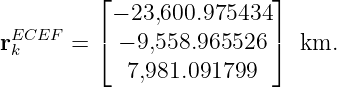
The final ECEF position is

x_k	= x′_k cos Ω_k − y′_k cos i_k sin Ω_k,	(45)
y_k	= x′_k sin Ω_k + y′_k cos i_k cos Ω_k,	(46)
z_k	= y′_k sin i_k.	(47)

Thus

⌊ ⌋ − 23,600.975434 rEkCEF = ⌈ − 9,558.965526 ⌉ km. 7,981.091799

(48)

5 Sheet 3: corrected CNAV velocity

Why an instantaneous n_k is required

Differentiating Equation (23) gives the instantaneous mean-anomaly rate

˙ Mk = nk = n0 + Δn0 + Δ ˙n0tk.

(49)

At two hours,

nk = 1.45859184447025 × 10−4 rad∕s.

(50)

This is distinct from the interval-average n_A used to produce M_k. RFC-00544 corrects the CNAV eccentric-anomaly-rate equation to use this instantaneous rate [2, 3].

Eccentric- and true-anomaly rates

Differentiating Kepler’s equation gives

n E˙k = ------k-----= 1.45178207569980 × 10 −4 rad ∕s. 1 − ecosEk

(51)

Then

√ ------ ˙ ---1-−-e2--- −4 ˙νk = Ek 1 − ecosEk = 1.44493184787688 × 10 rad ∕s.

(52)

For comparison, simply inserting the sheet-1 interval-average n_A in the numerator would give a slightly different Ė_k. The distinction is small numerically here but exact analytically.

Corrected inclination, latitude, and radius rates

The inclination rate is

dik dt-= IDOT + 2˙νk(Ciscos 2Φk − Cic sin 2Φk),

(53)

which gives

dik −10 --- = − 2.22868216 × 10 rad ∕s. dt

(54)

The corrected argument-of-latitude rate is

˙uk = ˙νk + 2˙νk(Cus cos2Φk − Cuc sin2Φk ),

(55)

u˙k = 1.44495076805993 × 10−4 rad∕s.

(56)

Because A_k is time varying, differentiation of

rk = Ak (1 − ecos Ek) + δrk

(57)

requires the product rule. With the RFC-00544 correction,

˙rk = A˙(1 − e cosEk ) + Ake sin Ek ˙Ek + 2˙νk(Crs cos2Φk − Crcsin2Φk ).

(58)

Numerically,

˙rk = 34.12570174 m ∕s.

(59)

Orbital-plane velocity

The Earth-fixed node rate is

Ω˙ = ˙Ω − Ω˙ = − 7.29291513866 × 10− 5 rad ∕s. k e

(60)

The in-plane rates are

x˙′= ˙r cosu − r u˙ sin u , k k k k k k

(61)

′ y˙k = r˙k sin uk + rk ˙uk cosuk.

(62)

which give

′ x˙k = − 1439.60291978 m ∕s,

(63)

′ ˙yk = − 3577.15739766 m ∕s.

(64)

For compactness define

di Qx = Ω˙k cos Ωk cosik − --ksinΩk sinik, dt

(65)

˙ dik Qy = Ωk sinΩk cos ik + dt cosΩk sinik.

(66)

Differentiating the ECEF position transformation then gives

′ ′ ′ ′ ˙xk = − xk ˙Ωk sin Ωk + x˙k cosΩk − ˙yk sinΩk cos ik − ykQx,

(67)

y˙k = x′k ˙Ωk cosΩk + ˙x′k sinΩk + ˙y′k cosΩk cos ik − yk′Qy,

(68)

dik z˙k = y˙′k sin ik + yk′--cos ik. dt

(69)

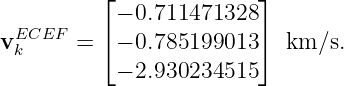
Therefore

⌊ ⌋ − 0.711471328 vEkCEF = ⌈− 0.785199013 ⌉ km ∕s. − 2.930234515

(70)

6 Sheet 4: ECEF acceleration

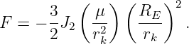
Table 30-II sheet 4 uses the corrected radius from sheet 2 and defines

( ) ( )2 F = − 3J2 -μ RE-- . 2 r2k rk

(71)

For this state,

F = − 5.19326591 × 10 −5 m∕s2.

(72)

The acceleration components are

( ) xk- z2k- xk- ˙ ˙ 2 ¨xk = − μ r3 + F 1 − 5r2 rk + 2˙ykΩe + xk(Ωe ) , k k

(73)

y ( z2) y ¨yk = − μ -k3-+ F 1 − 5-k2- --k− 2˙xk ˙Ωe + yk(Ω˙e )2, rk rk rk

(74)

( ) zk- z2k- zk- ¨zk = − μ r3 + F 3 − 5r2 rk. k k

(75)

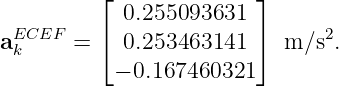
The result is

⌊ 0.255093631 ⌋ ECEF ⌈ ⌉ 2 a k = 0.253463141 m∕s . − 0.167460321

(76)

7 Verification checks

The calculation should not be trusted merely because the formulas run without an exception. Several independent checks are available.

Kepler residual

The converged eccentric anomaly satisfies

Mk − (Ek − esinEk ) = 0

(77)

to machine precision in the reference calculation.

Radius-preserving coordinate transformations

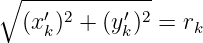
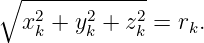
Because the orbital-plane and ECEF transformations are rotations,

∘ ------------- ′ 2 ′ 2 (xk) + (yk) = rk

(78)

and

∘ ------------ 2 2 2 xk + yk + zk = rk.

(79)

Both residuals are zero to displayed double-precision accuracy in the supplied script.

Finite-difference anomaly and radius rates

With a symmetric step h = 0.1 s,

˙ E(t +-h) −-E(t-−-h)- EF D = 2h

(80)

agrees with the analytical corrected CNAV rate to

|E ˙ − ˙E | ≈ 3.4 × 10−14 rad ∕s. FD k

(81)

Similarly,

| | |r(t + h ) − r (t − h) | ||-------------------− r˙k|| ≈ 2.3 × 10−8 m ∕s. 2h

(82)

Finite-difference ECEF velocity

The position algorithm alone gives an independent numerical velocity estimate,

r(t +-h-) −-r(t −-h) vF D = 2h .

(83)

The error norm is

∥vF D − vk∥ ≈ 8.72 × 10 −7 m∕s.

(84)

This is a strong end-to-end confirmation that the corrected n_k and A_k velocity terms are consistent with the CNAV position solution.

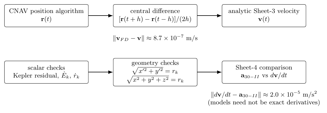
Figure 3. Independent checks used to validate the numerical CNAV implementation.

Why sheet-4 acceleration need not equal the exact derivative of sheet 3

A central difference of the analytical velocity gives an acceleration differing from the sheet-4 model by

∥ ∥ ∥∥ v(t +-h) −-v-(t −-h-)− a ∥∥ ≈ 2.03 × 10 −5 m∕s2. ∥ 2h 30− II∥

(85)

This is not evidence that the position or velocity derivation failed. Sheet 4 is a prescribed central-gravity plus J₂ rotating-Earth acceleration model. The fitted position and velocity equations include broadcast secular and harmonic terms, so sheet 4 is not constructed as the exact second derivative of every fitted coefficient appearing in sheets 1–3.

8 Matched LNAV-style comparison

To isolate the contribution of the CNAV-only secular terms, define a matched baseline that uses exactly the same reference-time geometry, eccentricity, harmonic coefficients, inclination rate, node rate, and epoch values, but suppresses

˙A = 0, Δ ˙n0 = 0.

(86)

The baseline then behaves like the legacy LNAV model with constant fitted semimajor axis and constant mean-motion correction:

AL = A0,

(87)

nL = n0 + Δn0,

(88)

ML = M0 + nLtk.

(89)

This is an intentionally controlled mathematical comparison, not a claim that the two broadcast messages for a real satellite would contain identical fitted values.

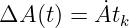
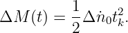
At the reference epoch, the two position solutions are identical. The two CNAV-only departures subsequently grow as

ΔA (t) = A˙tk

(90)

and

ΔM (t) = 1Δ ˙n0t2k. 2

(91)

At two hours,

ΔA = 107.9990 m,

(92)

while

−6 ΔM = − 7.77601 × 10 rad.

(93)

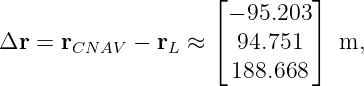
The resulting ECEF differences are

⌊ ⌋ − 95.203 Δr = rCNAV − rL ≈ ⌈ 94.751 ⌉ m, 188.668

(94)

with

∥Δr ∥ ≈ 231.597 m.

(95)

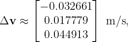
The velocity difference is

⌊ ⌋ − 0.032661 Δv ≈ ⌈ 0.017779 ⌉ m ∕s, 0.044913

(96)

− 2 ∥Δv ∥ ≈ 5.831 × 10 m ∕s.

(97)

The acceleration-model difference at the two propagated states is approximately

∥Δa ∥ ≈ 2.83 × 10−6 m ∕s2.

(98)

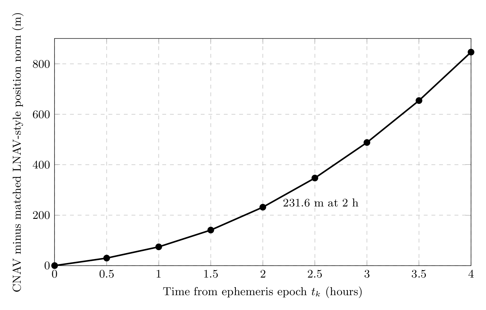
Figure 4. Growth of the ECEF position difference between the CNAV solution and the matched LNAV-style baseline.

The time history makes the structural difference clear:

t_k (h)	ΔA (m)	ΔM (rad)	∥Δr∥ (m)
0.0	0.000	0	0.000
0.5	27.000	−4.8600 × 10⁻⁷	29.760
1.0	54.000	−1.9440 × 10⁻⁶	74.336
1.5	80.999	−4.3740 × 10⁻⁶	140.864
2.0	107.999	−7.7760 × 10⁻⁶	231.597
2.5	134.999	−1.2150 × 10⁻⁵	347.231
3.0	161.999	−1.7496 × 10⁻⁵	488.072
3.5	188.998	−2.3814 × 10⁻⁵	654.372
4.0	215.998	−3.1104 × 10⁻⁵	846.429

This is the central numerical lesson of CNAV. The extra parameters do not redefine orbital mechanics; they allow the broadcast fit to carry low-order secular drift that a constant-A, constant-Δn legacy parameterization must absorb elsewhere in its finite-interval fit.

9 Implementation checklist

A robust CNAV implementation should perform the following operations in this order:

1.: Decode the Message type 10/11 fields and apply Table 30-I scale factors.
2.: Convert all semicircle-based angular quantities with the ICD value of π; do not multiply the radian harmonic coefficients by π.
3.: Form A₀ = AREF + ΔA and A_k = A₀ + Ȧt_k.
4.: Apply GPS-week crossover handling to t_k.
5.: Compute n₀ from A₀.
6.: Form the sheet-1 interval-average Δn_A and n_A, then compute M_k.
7.: Solve Kepler’s equation and compute ν_k with a quadrant-safe function.
8.: Evaluate the three second-harmonic corrections and form u_k,r_k,i_k.
9.: Reconstruct the full node rate from the CNAV reference node rate plus the transmitted node-rate difference, compute Ω_k, and obtain ECEF position.
10.: For velocity, form the instantaneous n_k from Equation (49), then use the RFC-00544 corrected Ė_k equation.
11.: Include both the explicit Ȧ(1 − e cos E_k) term and A_k in the corrected CNAV radius rate.
12.: Differentiate the orbital-plane and ECEF rotations to obtain velocity.
13.: Use sheet 4 for the prescribed Earth-fixed acceleration model.
14.: Run the residual, norm, scalar finite-difference, and vector finite-difference checks before trusting the result.

The supplied program GPSORB18_reference.py implements this sequence and writes three regression files: the complete intermediate-value list, the two-hour CNAV/LNAV-style comparison, and the four-hour comparison time history.

10 Summary

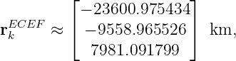
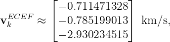
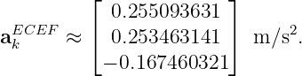
For the worked example, the complete CNAV solution at t_k = 7200 s is

⌊ ⌋ ECEF − 23600.975434 rk ≈ ⌈ − 9558.965526 ⌉ km, 7981.091799

(99)

⌊ ⌋ − 0.711471328 vECEF ≈ ⌈− 0.785199013 ⌉ km ∕s, k − 2.930234515

(100)

and

⌊ 0.255093631 ⌋ ECEF ⌈ ⌉ 2 a k ≈ 0.253463141 m∕s . − 0.167460321

(101)

The end-to-end position-to-velocity finite-difference test closes at the sub-micrometer-per-second level for the selected numerical step, while the deliberately matched LNAV-style solution differs by about 232 m after two hours and about 846 m after four hours. Those differences arise from the two CNAV secular freedoms isolated here: linear semimajor-axis drift and quadratic mean-anomaly curvature.

References

[1] U.S. Space Force, NAVSTAR GPS Space Segment/Navigation User Segment Interfaces, IS-GPS-200N, 1 August 2022, especially Tables 30-I and 30-II. https://www.gps.gov/sites/default/files/2025-07/IS-GPS-200N.pdf

[2] U.S. Space Force, PCN-IS-200N RFC-00544: Eccentric Anomaly Rate Fix and No Cost Items, public review change notice, 2025–2026. https://www.gps.gov/sites/default/files/2026-01/PCN_IS-200N-RFC544_20251006_PubRev_20250930%20-%20NAVSTAR%20GPS%20Space%20SegmentNavigation%20User%20Segment%20Interfaces_0.pdf

[3] U.S. Space Force, 2026 Public Interface Control Working Group Meeting Minutes, 16 June 2026. https://www.gps.gov/sites/default/files/2026-07/2026%20PICWG_Meeting_Minutes_202600708.pdf

[4] GPS.gov, Interface Control Documents and Interface Specifications, current public document index, accessed September 2026. https://www.gps.gov/interface-control-documents-icds-interface-specifications-iss

[5] E. D. Kaplan and C. J. Hegarty, eds., Understanding GPS/GNSS: Principles and Applications, 3rd ed., Artech House, 2017.

"Complete CNAV Numerical Solution: IS-GPS-200 Table 30-II from Broadcast Parameters to ECEF State" is owned by bloftin.
(view preamble)

1 Purpose and document status

2 Constants and worked-example parameters

3 Sheet 1: semimajor axis, mean motion, and anomaly

Reference-time semimajor axis

Time-varying semimajor axis

Computed reference mean motion

Revision-N interval-average mean-motion correction

Mean anomaly

Newton solution of Kepler’s equation

True anomaly

4 Sheet 2: corrected orbit geometry and ECEF position

5 Sheet 3: corrected CNAV velocity

Why an instantaneous nk is required

Eccentric- and true-anomaly rates

Corrected inclination, latitude, and radius rates

Orbital-plane velocity

6 Sheet 4: ECEF acceleration

7 Verification checks

Kepler residual

Radius-preserving coordinate transformations

Finite-difference anomaly and radius rates

Finite-difference ECEF velocity

Why sheet-4 acceleration need not equal the exact derivative of sheet 3

8 Matched LNAV-style comparison

9 Implementation checklist

10 Summary

References

References

Why an instantaneous n_k is required