Full Numerical GPS Broadcast Ephemeris Solution: From Decoded LNAV Parameters to ECEF Position, Velocity, and Acceleration

1 Purpose of GPSORB16

Kaplan and Hegarty summarize the GPS broadcast orbit algorithm as a short sequence that converts ephemeris parameters into an Earth-centered Earth-fixed satellite position. IS-GPS-200 provides the normative legacy LNAV equations in Table 20-IV. The preceding GPSORB articles derived each piece separately. This article now executes the complete chain with one consistent set of numbers.

The calculation is

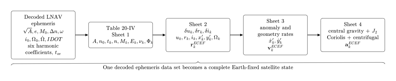
decoded LNAV ephemeris −→ rECEF −→ vECEF − → aECEF . k k k

(1)

Figure 1. The complete legacy LNAV orbit calculation from decoded ephemeris parameters through ECEF position, velocity, and acceleration.

The numerical values used here are deliberately illustrative rather than copied from one operational satellite message. They were chosen in GPSORB12–GPSORB15 to be GPS-like and to make every intermediate step transparent. The purpose is reproducibility of the mathematics, not reproduction of one historical SV state.

IS-GPS-200 states that the subframe 2 and 3 quantities are Keplerian in appearance but are generated from a least-squares fit to a propagated Earth-fixed trajectory. The user equations are therefore best understood as a compact fitted trajectory model rather than as an untouched six-element Kepler orbit [1].

2 Constants used by the GPS user algorithm

The legacy Table 20-IV computation uses

14 3 2 μ = 3.986005 × 10 m ∕s

(2)

and

˙Ωe = 7.2921151467 × 10−5 rad∕s.

(3)

For the acceleration calculation, sheet 4 additionally uses

R = 6378137.0 m, E

(4)

J2 = 0.0010826262.

(5)

Because the satellite position is extremely sensitive to small angular errors, IS-GPS-200N also specifies the value

π = 3.1415926535898

(6)

for use in the broadcast ephemeris calculation [1].

3 Decoded parameters and computation units

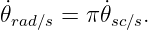
The user equations are applied after the navigation bits have been decoded and their LSB scale factors applied. Some decoded angular quantities are expressed in semicircles, whereas the trigonometric and differential equations are most naturally evaluated in radians. Therefore

𝜃 = π𝜃 rad sc

(7)

and

𝜃˙rad∕s = π ˙𝜃sc∕s.

(8)

The harmonic coefficients C_uc,C_us,C_ic,C_is are already specified in radians and should not receive another factor of π [1].

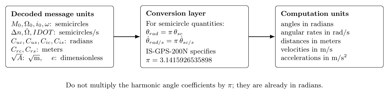
Figure 2. Unit conversion should be completed before entering the numerical orbit equations.

For the worked example, all angular quantities below are listed directly in the computation units used by the equations.

Core ephemeris and timing values

Parameter	Value used	Computation units
	5153.63949069
e	0.010000	dimensionless
Δn	4.5 × 10⁻⁹	rad/s
M₀	1.000000	rad
ω	0.700000	rad
t_oe	345600	s
t	352800	s
i₀	0.95993108860	rad
Ω₀	1.200000	rad
dΩ∕dt	−8.0 × 10⁻⁹	rad/s
IDOT	−2.0 × 10⁻¹⁰	rad/s

Harmonic correction coefficients

Parameter	Value used	Units
C_us	8.0 × 10⁻⁶	rad
C_uc	1.0 × 10⁻⁶	rad
C_rs	80	m
C_rc	200	m
C_is	−2.0 × 10⁻⁷	rad
C_ic	1.0 × 10⁻⁷	rad

The evaluation epoch was chosen so that

t − toe = 7200 s,

(9)

which is comfortably inside the half-week crossover boundary.

4 Sheet 1: time and anomaly propagation

1. Semimajor axis

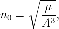
The message transmits √ --
A , so

A = (√A--)2.

(10)

Numerically,

2 A = (5153.63949069 ) ,

(11)

therefore

A = 2.6560000 × 107 m = 26560 km.

(12)

2. Computed mean motion

∘ ---- n = μ--, 0 A3

(13)

−4 n0 = 1.4585684444 × 10 rad∕s.

(14)

3. Time from ephemeris epoch

tk = t − toe = 352800 − 345600,

(15)

thus

tk = 7200 s.

(16)

IS-GPS-200 requires half-week crossover correction if t_k exceeds +302400 s or falls below −302400 s. No correction is needed here [1].

4. Corrected mean motion

n = n0 + Δn,

(17)

which yields

n = 1.4586134444 × 10− 4 rad ∕s.

(18)

5. Mean anomaly

Mk = M0 + ntk,

(19)

therefore

Mk = 2.05020167997 rad.

(20)

6. Eccentric anomaly

Kepler’s equation is

Mk = Ek − esin Ek.

(21)

Following Table 20-IV, initialize

E0 = Mk

(22)

and apply

Mk-−-Ej-−1-+-esinEj-−1- Ej = Ej− 1 + 1 − ecos Ej−1 .

(23)

The three required refinements give

E1 = 2.05903363604 rad,

(24)

E2 = 2.05903329214 rad,

(25)

E = 2.05903329214 rad. 3

(26)

Hence

Ek = 2.05903329214 rad.

(27)

7. True anomaly and argument of latitude

A quadrant-safe form is

(√ -----2 ) νk = atan2 1 − e sinEk, cosEk − e ,

(28)

which gives

νk = 2.06784440233 rad.

(29)

Then

Φk = νk + ω,

(30)

Φk = 2.76784440233 rad.

(31)

5 Sheet 2: corrected orbit geometry and ECEF position

The twice-per-revolution phase is

2Φk = 5.53568880466 rad.

(32)

The three harmonic corrections are

δuk = Cus sin2Φk + Cuccos 2Φk,

(33)

δrk = Crs sin2Φk + Crccos 2Φk,

(34)

δi = C sin 2Φ + C cos2Φ . k is k ic k

(35)

Numerically,

δuk = − 4.70504570 × 10−6 rad,

(36)

δrk = 92.2942234 m,

(37)

and

δik = 2.09300274 × 10−7 rad.

(38)

The corrected quantities become

uk = Φk + δuk,

(39)

rk = A(1 − ecos Ek) + δrk,

(40)

ik = i0 + IDOT tk + δik.

(41)

Thus

uk = 2.76783969728 rad,

(42)

rk = 2.66846771731 × 107 m,

(43)

and

ik = 0.959929857897 rad.

(44)

The corrected orbital-plane coordinates are

x′= rk cos uk, y′ = rk sin uk, k k

(45)

′ 7 x k = − 2.48424646234 × 10 m,

(46)

y ′k = 9.74289214087 × 106 m.

(47)

The Earth-fixed node longitude is

Ωk = Ω0 + (˙Ω − ˙Ωe)tk − ˙Ωetoe.

(48)

For this example,

Ωk = − 24.5266398376 rad.

(49)

The equivalent wrapped angle is

Ω ≡ 0.60610139116 rad (mod 2π). k

(50)

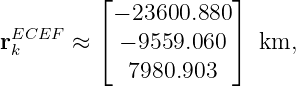
The final WGS 84 ECEF position is

′ ′ xk = x k cosΩk − yk cos ik sin Ωk,

(51)

yk = x ′k sin Ωk + y ′k cosik cos Ωk,

(52)

zk = y′k sin ik.

(53)

Hence

⌊ ⌋ − 2.36008802326 × 107 rEkCEF = ⌈ − 9.55906026760 × 106⌉ m. 7.98090313697 × 106

(54)

6 Sheet 3: analytical ECEF velocity

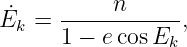
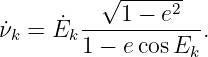
Differentiate Kepler’s equation to obtain

n ˙Ek = ------------, 1 − e cosEk

(55)

and then

√ ------ ˙ ----1-−-e2-- ˙νk = Ek1 − e cosE . k

(56)

For the example,

−4 E˙k = 1.45180347602 × 10 rad ∕s,

(57)

ν˙k = 1.44495304892 × 10− 4 rad∕s.

(58)

The corrected inclination, argument-of-latitude, radius, and node rates are

˙ik = IDOT + 2˙νk (Cis cos2Φk − Cic sin 2Φk ),

(59)

u˙k = ˙νk + 2 ˙νk (Cus cos2Φk − Cuc sin2Φk ),

(60)

˙rk = Ae ˙Ek sin Ek + 2ν˙k (Crscos 2Φk − Crc sin 2Φk) ,

(61)

and

Ω˙ = ˙Ω − Ω˙ . k e

(62)

Numerically,

˙ik = − 2.22743020 × 10−10 rad∕s,

(63)

˙uk = 1.44497196899 × 10− 4 rad ∕s,

(64)

˙rk = 34.1108554 m∕s,

(65)

˙Ωk = − 7.2929151467 × 10−5 rad∕s.

(66)

The in-plane velocity components are

x˙′= ˙rk cosuk − rku˙k sin uk, k

(67)

′ y˙k = r˙k sin uk + rk ˙uk cosuk,

(68)

which give

˙x′k = − 1439.576571 m ∕s,

(69)

˙y′k = − 3577.212224 m ∕s.

(70)

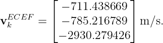
Substitution into the full Table 20-IV sheet-3 product-rule equations yields

⌊ ⌋ − 711.438669 vEkCEF = ⌈ − 785.216789 ⌉ m ∕s. − 2930.279426

(71)

The ECEF speed is

∥vEkCEF ∥ ≈ 3.11597 km ∕s.

(72)

7 Sheet 4: ECEF acceleration

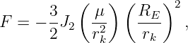
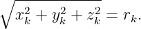
A useful notation point is important here. Sheet 4 uses the corrected r_k already computed on sheet 2. The identity

∘ --2---2----2 x k + yk + zk = rk

(73)

is therefore best treated as a numerical consistency check, not as a new definition of r_k.

The oblate-Earth acceleration factor is

3 ( μ ) ( R )2 F = − -J2 -2 -E-- , 2 rk rk

(74)

which gives

F = − 5.19334896206 × 10− 5 m ∕s2.

(75)

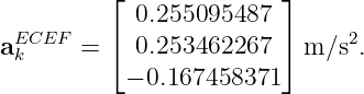
The final Table 20-IV acceleration equations are

( ) xk- z2k- xk- 2 ¨xk = − μ r3 + F 1 − 5r2 r + 2y˙kΩ˙e + xk ˙Ωe, k k k

(76)

( 2) ¨y = − μ yk-+ F 1 − 5zk- yk-− 2˙x Ω˙ + y Ω˙2 , k r3k r2k rk k e k e

(77)

zk ( z2) zk ¨zk = − μ-3-+ F 3 − 5-k2- --. rk rk rk

(78)

They produce

⌊ ⌋ 0.255095487 aEkCEF = ⌈ 0.253462267 ⌉ m ∕s2. − 0.167458371

(79)

The component breakdown is

Contribution	x (m/s²)	y (m/s²)	z (m/s²)
Central gravity	+0.49508547	+0.20052438	−0.16741872
J₂ gravity	+0.00002539	+0.00001028	−0.00003965
Coriolis	−0.11451782	+0.10375785	0
Centrifugal	−0.12549755	−0.05083025	0
Final ECEF	+0.25509549	+0.25346227	−0.16745837

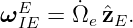
To keep scalar and vector Earth-rotation notation distinct, the rotating-frame derivation may write

E ω IE = Ω˙e ˆzE.

(80)

Then

( ) aE = aEg − 2ωEIE × vE − ωEIE × ωEIE × rE ,

(81)

which is the vector form behind the Coriolis and centrifugal terms above.

8 The complete output state

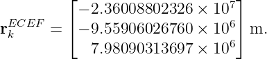
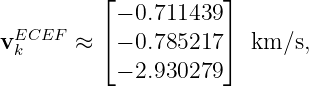
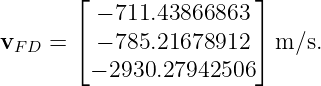
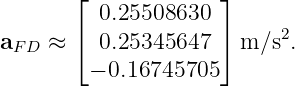
The entire worked solution may now be summarized as

⌊ ⌋ − 23600.880 rEkCEF ≈ ⌈ − 9559.060 ⌉ km, 7980.903

(82)

⌊ ⌋ − 0.711439 vEkCEF ≈ ⌈ − 0.785217 ⌉ km ∕s, − 2.930279

(83)

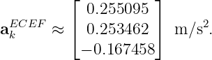
and

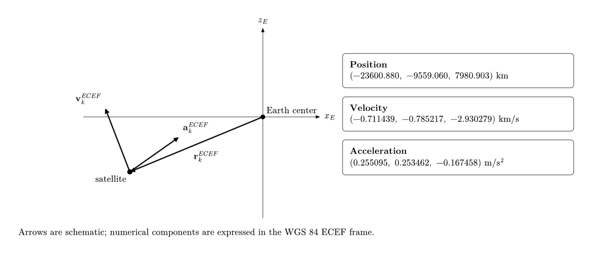
⌊ ⌋ 0.255095 aECEF ≈ ⌈ 0.253462 ⌉ m ∕s2. k − 0.167458

(84)

Figure 3. Final position, velocity, and acceleration from the worked broadcast ephemeris. Vector directions in the sketch are schematic.

9 Intermediate-value audit table

The following condensed table is useful when debugging an independent implementation.

Stage	Quantity	Numerical value
Sheet 1	A	2.6560000 × 10⁷ m
	n₀	1.4585684444 × 10⁻⁴ rad/s
	t_k	7200 s
	n	1.4586134444 × 10⁻⁴ rad/s
	M_k	2.05020167997 rad
	E_k	2.05903329214 rad
	ν_k	2.06784440233 rad
	Φ_k	2.76784440233 rad
Sheet 2	δu_k	−4.70504570 × 10⁻⁶ rad
	δr_k	92.2942234 m
	δi_k	2.09300274 × 10⁻⁷ rad
	u_k	2.76783969728 rad
	r_k	2.66846771731 × 10⁷ m
	i_k	0.959929857897 rad
	Ω_k	−24.5266398376 rad
Sheet 3	dE_k∕dt	1.45180347602 × 10⁻⁴ rad/s
	dν_k∕dt	1.44495304892 × 10⁻⁴ rad/s
	dr_k∕dt	34.1108554 m/s
	du_k∕dt	1.44497196899 × 10⁻⁴ rad/s
	dΩ_k∕dt	−7.2929151467 × 10⁻⁵ rad/s
Sheet 4	F	−5.19334896206 × 10⁻⁵ m/s²

The companion file GPSORB16_intermediates.csv contains a longer machine-readable version of this table.

10 Verification: do not trust a long chain without checks

An end-to-end ephemeris calculation has enough trigonometric signs, unit conversions, and frame conventions that verification should be designed into the implementation.

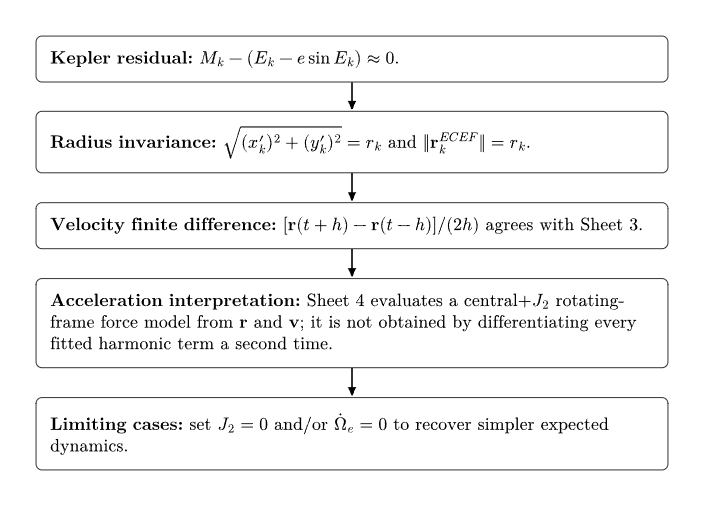
Figure 4. A practical hierarchy of checks for a broadcast ephemeris implementation.

1. Kepler residual

After the third Newton refinement, evaluate

𝜖K = Mk − (Ek − e sin Ek).

(85)

For the numerical precision shown here,

𝜖K ≈ 0.

(86)

A non-negligible residual immediately indicates a Kepler-solver problem.

2. Orbital-plane radius check

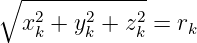
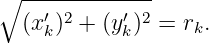
Because

′ ′ xk = rk cos uk, yk = rk sin uk,

(87)

we must have

∘ ------------- (x′k)2 + (y′k)2 = rk.

(88)

3. ECEF radius check

The transformation from corrected orbital-plane coordinates to ECEF is a rotation, so it preserves length:

∘ ------------ x2 + y2 + z2 = rk. k k k

(89)

This check is particularly effective for detecting sign mistakes in Ω_k or inclination.

4. Finite-difference velocity

Evaluate the complete sheet-1/sheet-2 position algorithm at t − h and t + h and form

r(t + h ) − r(t − h) vF D = ------------------. 2h

(90)

With

h = 0.1 s,

(91)

the numerical result is approximately

⌊ ⌋ − 711.43866863 vF D = ⌈ − 785.21678912 ⌉ m∕s. − 2930.27942506

(92)

The difference from the analytic sheet-3 velocity has norm

ECEF −7 ∥vFD − vk ∥ ≈ 9.1 × 10 m ∕s.

(93)

This is a stringent end-to-end check of the Sheet-2 geometry and Sheet-3 derivatives.

5. Why the Sheet-4 acceleration need not equal a second numerical derivative exactly

There is an important conceptual distinction between sheets 3 and 4. Sheet 3 is obtained by differentiating the broadcast position expressions. Sheet 4, however, evaluates a separate central-gravity plus J₂ rotating-frame acceleration model from the already computed position and velocity. The ICD does not obtain sheet 4 by differentiating every fitted harmonic term a second time.

For the illustrative data set, differentiating the sheet-3 velocity numerically with h = 0.1 s gives approximately

⌊ 0.25508630 ⌋ ⌈ ⌉ 2 aF D ≈ 0.25345647 m ∕s . − 0.16745705

(94)

The difference from the Table 20-IV sheet-4 acceleration has magnitude

∥aFD − aSheet4∥ ≈ 1.09 × 10−5 m ∕s2.

(95)

This small mismatch is not a sign error. The broadcast parameters are fitted coefficients for an ECEF trajectory, while sheet 4 is a compact force-model acceleration expression [1]. The two calculations answer closely related but not algebraically identical questions.

6. Limiting-case checks

Several switches provide useful unit tests:

Set all six harmonic coefficients to zero. The sheet-2 corrections must disappear.
Set Δn = 0. Mean motion must reduce to n₀.
Set IDOT = 0 and the inclination harmonic coefficients to zero. Then i_k = i₀ and the inclination rate is zero.
Set J₂ = 0. The oblate-Earth term must disappear from sheet 4.
Set the Earth rotation rate to zero. Coriolis and centrifugal terms must vanish and the node equation loses Earth-rotation terms.

11 Implementation ordering

A receiver or analysis script can implement the complete orbit calculation in the following order:

1.: Decode the LNAV ephemeris parameters and apply their LSB scale factors.
2.: Convert semicircle-based angles and angular rates to radians using Equation (6).
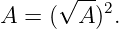
3.: Form A = ()² and n₀ = .
4.: Compute t_k = t − t_oe and apply the half-week crossover rule.
5.: Form n = n₀ + Δn and M_k = M₀ + nt_k.
6.: Solve Kepler’s equation for E_k using at least three Newton refinements.
7.: Compute ν_k with an unambiguous quadrant and form Φ_k = ν_k + ω.
8.: Evaluate δu_k, δr_k, and δi_k.
9.: Form corrected u_k, r_k, and i_k.
10.: Compute x′_k, y′_k, and Ω_k.
11.: Rotate into x_k,y_k,z_k ECEF coordinates.
12.: Evaluate the sheet-3 rates and obtain the three ECEF velocity components.
13.: Reuse the corrected sheet-2 r_k, compute F, and evaluate sheet-4 acceleration.
14.: Run the residual and norm checks before using the state in a navigation solution.

12 Reference implementation and data files

The companion script GPSORB16_reference.py implements the complete worked example using only the Python standard library. It also writes two CSV files:

GPSORB16_input_ephemeris.csv, containing the decoded example parameters in computation units;
GPSORB16_intermediates.csv, containing the intermediate and final numerical values.

These files are intended as regression-test data. A new C, C++, MATLAB, Julia, or embedded receiver implementation should reproduce the same values to the precision appropriate to its floating-point arithmetic.

13 Connection back to Kaplan’s Table 2.3

Kaplan’s Table 2.3 emphasizes the position calculation. The sequence

′ ′ A → n → tk → Mk → Ek → νk → Φk → (uk, rk,ik) → (xk,yk) → Ωk → (xk,yk,zk)

(96)

is precisely the core GPS broadcast position computation. GPSORB12 and GPSORB13 derived that chain in the notation of the modern public interface specification. GPSORB14 and GPSORB15 then continued beyond Kaplan’s position table to the velocity and acceleration equations now supplied in Table 20-IV.

This completes the conceptual path that motivated GPSORB00:

μ- ¨r = − r3r =⇒ six orbital constants = ⇒ broadcast ephemeris =⇒ (r,v,a )ECEF .

(97)

14 Summary

One legacy LNAV ephemeris data set, after decoding and unit conversion, is sufficient to drive the complete Table 20-IV calculation. For the illustrative GPS-like parameters used throughout GPSORB12–GPSORB16, the final Earth-fixed state is

rECEF ≈ (− 23600.880,− 9559.060, 7980.903) km, k

(98)

ECEF v k ≈ (− 0.711439, − 0.785217,− 2.930279 ) km ∕s,

(99)

and

aECkEF ≈ (0.255095, 0.253462, − 0.167458 ) m ∕s2.

(100)

The important lesson is not the particular numbers. It is the chain of models behind them: Newtonian two-body mechanics, orbital elements, anomaly propagation, fitted harmonic corrections, Earth rotation, analytical differentiation, and finally a compact J₂ rotating-frame acceleration model. That chain is what turns a small set of broadcast coefficients into a satellite state usable by a GPS receiver.

References

[1] Global Positioning Systems Directorate, IS-GPS-200N: NAVSTAR GPS Space Segment/Navigation User Interfaces, 1 August 2022, especially Section 20.3.3.4.3 and Tables 20-III and 20-IV. Available from GPS.gov.

[2] GPS.gov, Interface Control Documents (ICDs) and Interface Specifications (ISs), current public-document index, accessed September 2026.

[3] E. D. Kaplan and C. J. Hegarty, eds., Understanding GPS: Principles and Applications, 2nd ed., Artech House, 2006, Chapter 2.

[4] E. D. Kaplan and C. J. Hegarty, eds., Understanding GPS/GNSS: Principles and Applications, 3rd ed., Artech House, 2017.

[5] D. A. Vallado, Fundamentals of Astrodynamics and Applications, 4th ed., Microcosm Press, 2013.

"Full Numerical GPS Broadcast Ephemeris Solution: From Decoded LNAV Parameters to ECEF Position, Velocity, and Acceleration" is owned by bloftin.
(view preamble)