From LNAV to CNAV: The Modernized GPS Broadcast Ephemeris and the 2026 Eccentric-Anomaly-Rate Correction

1 Why GPSORB17 comes after the legacy LNAV sequence

GPSORB16 closed the original path from Newton’s equation

μ- ¨r = − r3r

(1)

through the six classical orbital elements and finally through the four sheets of the legacy LNAV user algorithm. The natural extension is the modernized Civil Navigation message, or CNAV.

CNAV does not replace orbital mechanics with a different theory. It keeps the same conic geometry, Kepler equation, second-harmonic corrections, orbital-plane coordinates, Earth-fixed transformation, velocity equations, and J₂ acceleration structure. The main conceptual change is that the fitted reference orbit is allowed to evolve more explicitly in time.

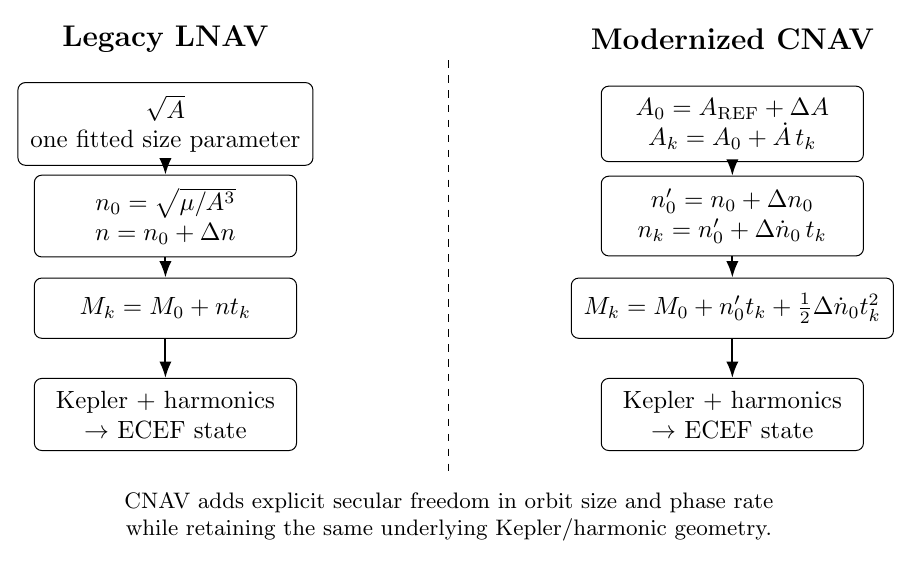
Figure 1. Legacy LNAV and modernized CNAV use the same orbital geometry, but CNAV adds explicit secular freedom in semimajor axis and mean-motion rate.

The public IS-GPS-200N specification places the CNAV ephemeris parameters in Message types 10 and 11 and gives the user equations in Table 30-II [1]. The current GPS.gov document index, as of September 2026, still lists IS-GPS-200N together with IRN-003 and IRN-004 as the issued public baseline [4].

2 The key CNAV parameters

The CNAV orbit model introduces four parameters that deserve special attention:

ΔA, A˙, Δn , Δ ˙n . 0 0

(2)

Table 30-I defines ΔA as a semimajor-axis difference relative to the fixed reference value

AREF = 26,559,710 m.

(3)

It defines the transmitted semimajor-axis rate as the change rate of the fitted size, Δn₀ as the mean-motion difference at the reference time, and the transmitted mean-motion-difference rate as its time derivative [1].

The node rate is treated similarly. CNAV broadcasts a difference relative to

˙ −9 ΩREF = − 2.6 × 10 semicircles/s.

(4)

Thus reference-centered coding is used both for orbital size and for the right-ascension rate.

This is a useful engineering idea. Instead of spending bits representing the full value of a quantity known to be close to a Constellation nominal value, CNAV can transmit a smaller departure from a reference.

3 CNAV semimajor axis: from a constant fitted size to a linear model

The first CNAV equation is

A0 = AREF + ΔA.

(5)

Here A₀ is the semimajor axis at the ephemeris reference time t_oe.

Define

tk = t − toe,

(6)

with the same week-crossover handling used in the legacy algorithm. CNAV then allows the fitted semimajor axis to drift linearly:

Ak = A0 + A˙tk.

(7)

Differentiating Equation (7) immediately gives

dAk- ˙ dt = A.

(8)

This looks simple, but it has an important consequence later. The radius model contains A_k, so the radius rate must contain an explicit semimajor-axis-rate contribution. That term does not exist in legacy LNAV because its fitted semimajor axis is constant over the user model interval.

4 Reference mean motion

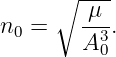
CNAV computes the Keplerian reference mean motion from A₀:

∘ ---- n0 = μ--. A30

(9)

Notice the modeling choice: the mean-motion baseline is formed from the semimajor axis at the reference epoch, A₀, rather than recomputed continuously from A_k.

This is appropriate because the CNAV message is a fitted parameterization. The transmitted mean-motion difference and its rate provide independent freedom to fit the along-track phase evolution instead of forcing it to follow only the instantaneous Kepler relation n ∝ A^−3∕2.

Define the corrected mean motion at reference time

n′0 = n0 + Δn0.

(10)

The modernized time-dependent mean motion is then

nk = n ′0 + Δ n˙0 tk.

(11)

Thus CNAV has an explicit first-order model for the phase rate.

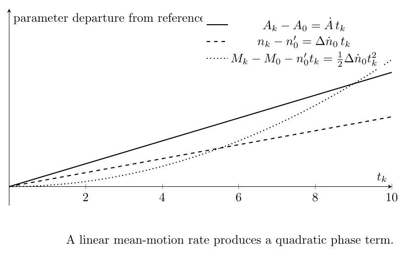
Figure 2. CNAV gives the broadcast fit a linear semimajor-axis drift, a linear mean-motion drift, and therefore a quadratic accumulated phase term.

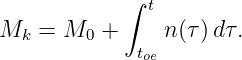
5 Deriving the CNAV mean anomaly

Mean anomaly is the accumulated phase associated with mean motion. Therefore the most fundamental statement is

∫ t Mk = M0 + n(τ)d τ. toe

(12)

With

n(τ) = n ′0 + Δ n˙0(τ − toe),

(13)

let

s = τ − toe.

(14)

Then Equation (12) becomes

∫ tk M = M + (n′ + Δ ˙n s)ds. k 0 0 0 0

(15)

Integrating term by term,

′ 1 2 Mk = M0 + n0tk + --Δn˙0tk. 2

(16)

The factor 1∕2 is not arbitrary. It is the inevitable result of integrating a linearly changing mean motion.

Equation (16) also gives the most important derivative identity in this article:

M˙k = n ′0 + Δ ˙n0tk = nk.

(17)

6 How Revision N packages the same phase law

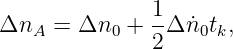
The published IS-GPS-200N Table 30-II sheet 1 expresses the mean-motion correction as

1- ΔnA = Δn0 + 2Δ n˙0tk,

(18)

and then defines

nA = n0 + ΔnA,

(19)

followed by

Mk = M0 + nAtk.

(20)

Substitution gives

( ) 1- Mk = M0 + n0 + Δn0 + 2Δ ˙n0tk tk,

(21)

1 Mk = M0 + (n0 + Δn0 )tk +--Δ ˙n0t2k. 2

(22)

Therefore the published sheet-1 expression gives the same mean anomaly as Equation (16).

The subtle problem appears only when a rate is needed. The quantity n_A above contains half of the accumulated linear-rate correction and therefore behaves like the average mean motion over the interval, not the instantaneous mean-anomaly derivative.

Indeed,

M˙ = n + Δn + Δ n˙t , k 0 0 0k

(23)

whereas

nA = n0 + Δn0 + 1Δ ˙n0tk. 2

(24)

They are equal only when

Δ n˙t = 0. 0 k

(25)

7 Kepler’s equation is unchanged

Once M_k has been formed, CNAV returns to the same ellipse geometry developed in GPSORB06 and used by LNAV:

Mk = Ek − esin Ek.

(26)

The usual Newton iteration applies:

E0 = Mk,

(27)

Ej = Ej− 1 + Mk-−-Ej-−1-+-esinEj-−1. 1 − ecos Ej−1

(28)

True anomaly is again obtained from E_k and e. A quadrant-safe implementation is

( ------ ) ν = atan2 √ 1 − e2sinE ,cosE − e . k k k

(29)

Thus the CNAV extension changes the time law feeding Kepler’s equation, not the conic geometry itself.

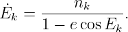
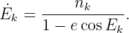
8 Deriving the eccentric-anomaly rate

Differentiate Kepler’s equation, Equation (26):

˙ ˙ ˙ Mk = Ek − ecos Ek Ek.

(30)

Factor the eccentric-anomaly rate:

M˙k = (1 − e cosEk ) ˙Ek.

(31)

Using Equation (17),

˙Ek = -----nk-----. 1 − e cosEk

(32)

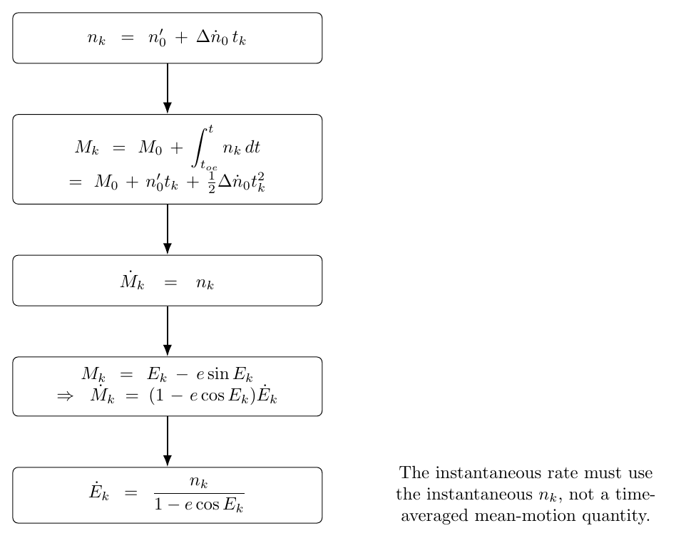
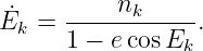
Figure 3. The corrected CNAV eccentric-anomaly rate follows directly by differentiating the quadratic mean-anomaly model.

This derivative is mathematically unavoidable once CNAV contains a nonzero mean-motion-difference rate.

9 The published Table 30-II issue and RFC-00544

The published 2022 IS-GPS-200N Table 30-II sheet 3 gives the CNAV eccentric-anomaly rate in a form using n rather than an explicitly defined instantaneous n_k [1]. In 2025–2026, the GPS public-interface process identified this as a CNAV formula error. The RFC-00544 proposed change notice states that the eccentric-anomaly-rate formulas in the CNAV public documents are incorrect and proposes a correction [2].

The correction reorganizes sheet 1 around

′ n0 = n0 + Δn0,

(33)

′ nk = n0 + Δn˙0tk,

(34)

and

Mk = M0 + n′0tk + 1-Δn˙0t2k, 2

(35)

so that sheet 3 can use the unambiguous rate

˙ -----nk----- Ek = 1 − e cosEk .

(36)

The June 2026 Public ICWG meeting minutes report that RFC-00544 was reviewed, that the substantive changes were accepted, and that the stakeholder comments were concurred with by the participating groups [3]. However, the current GPS.gov interface-document index still lists only IS-GPS-200N with IRN-003 and IRN-004 as issued changes [4]. Therefore this article distinguishes carefully between the published Revision-N baseline and the 2026 accepted correction language pending incorporation into a formally issued public baseline.

10 Why the correction matters physically

Suppose

Δ ˙n0 ⁄= 0.

(37)

Then the mean-motion correction changes linearly with time. The accumulated mean anomaly contains a quadratic term,

1 2 2Δ ˙n0tk,

(38)

but the instantaneous slope of that quadratic term is

Δ n˙0tk.

(39)

Using one-half of that slope in the eccentric-anomaly rate would be equivalent to confusing the average slope over the interval with the slope at the endpoint. The correction is therefore not merely a change in notation; it restores the derivative relationship

M˙k = (1 − e cosEk ) ˙Ek.

(40)

11 The CNAV radius and its rate

Ignoring the second-harmonic radial correction momentarily, CNAV uses

r = A (1 − e cosE ). k k k

(41)

Because both A_k and E_k depend on time, the product rule is required:

r˙k = A˙k (1 − ecos Ek) + Ak d-(1 − ecos Ek). dt

(42)

Since

A˙ = ˙A k

(43)

and

-d(1 − e cosEk ) = e sin Ek E˙k, dt

(44)

we obtain

˙r = A˙(1 − e cosE ) + A esinE E˙ . base k k k k

(45)

This is another place where CNAV differs from LNAV. Legacy LNAV has no explicit semimajor-axis-rate term.

When the radial harmonic correction

δr = C sin2 Φ + C cos 2Φ k rs k rc k

(46)

is included. Using the phase-rate identity from GPSORB14, differentiation gives

d -- δrk = 2˙νk (Crs cos2Φk − Crcsin2 Φk). dt

(47)

Therefore

r˙k = A˙(1 − ecos Ek) + Ake sinEk E˙k + 2˙νk (Crs cos2Φk − Crcsin2Φk ).

(48)

RFC-00544 also corrects the CNAV radius-rate equation so that the second term contains the time-varying A_k rather than an ambiguous A [2].

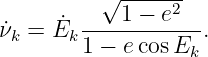
12 True-anomaly, inclination, and argument-of-latitude rates

The true-anomaly derivative remains

√ ------ ˙ ----1-−-e2-- ˙νk = Ek1 − e cosEk .

(49)

The inclination and argument-of-latitude rates retain the same harmonic derivative structure derived in GPSORB14:

˙ik = IDOT + 2˙νk (Cis cos2Φk − Cic sin 2Φk ),

(50)

u˙k = ˙νk + 2 ˙νk (Cus cos2Φk − Cuc sin2Φk ).

(51)

The modernized secular terms feed these equations mainly through the corrected anomaly rates and the time-varying radius.

13 The CNAV node-rate reference

CNAV does not broadcast the complete right-ascension rate directly. Instead it broadcasts a difference, which after unit conversion is combined with the fixed reference rate:

Ω˙ = ˙ΩREF + Δ ˙Ω.

(52)

The Earth-fixed ascending-node longitude then uses the same structure familiar from LNAV:

˙ ˙ ˙ Ωk = Ω0 −n + (Ω − Ωe )tk − Ωetoe.

(53)

The ECEF node rate is therefore

˙ ˙ ˙ Ωk = Ω − Ωe.

(54)

Again, the physics is not different. CNAV simply centers the encoded rate around a useful nominal reference.

14 What remains unchanged from LNAV

After CNAV forms the updated secular quantities, the rest of the orbit computation is strikingly familiar:

Φ = ν + ω , k k n

(55)

δuk = Cus− nsin2Φk + Cuc−n cos2Φk,

(56)

δr = C sin2Φ + C cos 2Φ , k rs− n k rc−n k

(57)

δik = Cis−n sin 2Φk + Cic− ncos2 Φk,

(58)

uk = Φk + δuk,

(59)

rk = Ak (1 − encos Ek) + δrk,

(60)

i = i + IDOT t + δi , k 0−n k k

(61)

x′k = rk cos uk, y′k = rk sin uk.

(62)

The final Earth-fixed coordinates remain

xk = x ′k cosΩk − y′k cos ik sin Ωk,

(63)

yk = x ′k sin Ωk + y ′k cosik cos Ωk,

(64)

zk = y′k sin ik.

(65)

The Table 30-II acceleration sheet also retains the same central-gravity, J₂, Coriolis, and centrifugal structure as Table 20-IV [1].

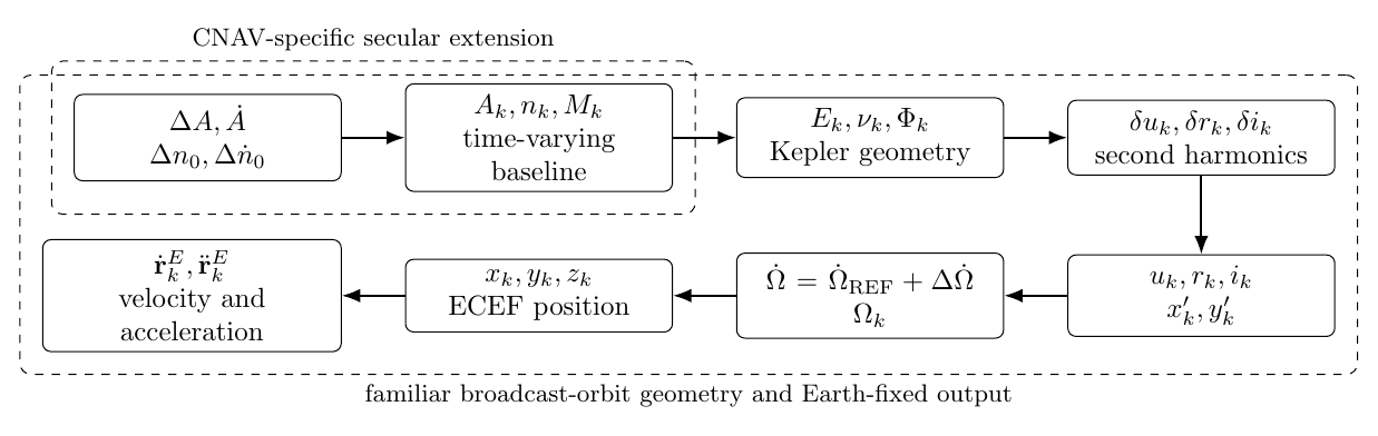
Figure 4. CNAV extends the secular baseline while retaining the familiar Kepler, harmonic, and ECEF portions of the broadcast-orbit calculation.

15 LNAV and CNAV compared directly

Concept	Legacy LNAV	Modernized CNAV
Semimajor-axis encoding	Full fitted size through square-root A	Difference from a fixed reference size
Semimajor-axis time law	Constant fitted size	Linear size drift
Mean-motion correction	One constant correction	Reference correction plus correction rate
Mean anomaly	Linear in elapsed time	Includes a quadratic elapsed-time term
Node-rate encoding	Full fitted node rate	Difference from a fixed reference rate
Kepler equation	Same ellipse equation	Same ellipse equation
Harmonic corrections	Three sine/cosine pairs	Same structure
ECEF position rotation	Same geometry	Same geometry
Velocity	No size-rate contribution	Explicit size-rate contribution to radial velocity
Acceleration	Central gravity, J2, and rotating-frame terms	Same structure

The table shows why CNAV should be viewed as a refinement of the broadcast fit, not as a new orbital theory.

16 A compact numerical example

Consider a synthetic GPS-like CNAV data set in computation units:

AREF = 26,559,710 m, ΔA = 290 m,

(66)

A˙= 0.015 m ∕s, tk = 7200 s,

(67)

Δn0 = 4.5 × 10 −9 rad∕s,

(68)

Δ ˙n = − 3.0 × 10−13 rad ∕s2, 0

(69)

and let

M0 = 1.0 rad, e = 0.01.

(70)

Equation (5) gives

A0 = 26,560,000 m.

(71)

After two hours,

Ak = 26,560,108 m.

(72)

The Keplerian reference mean motion is

n ≈ 1.4585684444 × 10−4 rad∕s. 0

(73)

The corrected reference value is

′ −4 n0 ≈ 1.4586134444 × 10 rad∕s,

(74)

and the instantaneous mean motion at t_k = 7200 s is

−4 nk ≈ 1.4585918444 × 10 rad∕s.

(75)

The mean anomaly becomes

Mk ≈ 2.05019390397 rad.

(76)

Newton iteration gives

Ek ≈ 2.05902555244 rad.

(77)

The corrected eccentric-anomaly rate is then

E˙ ≈ 1.45178207564 × 10 −4 rad ∕s. k

(78)

For comparison, if one incorrectly used the Revision-N interval-averaged quantity n_A as the instantaneous numerator, the result would be

˙(nA) −4 Ek ≈ 1.45179282522 × 10 rad∕s,

(79)

a difference of approximately

1.07 × 10 −9 rad∕s.

(80)

The number is small for this deliberately mild example, but the calculus distinction is exact and matters for a normative velocity equation.

Using Equation (45), the unperturbed radius rate is

˙rbase ≈ 34.07 m ∕s.

(81)

The explicit semimajor-axis-rate term contributes directly to this result.

17 Why extra broadcast coefficients do not add physical state dimensions

GPSORB02 showed that a satellite’s instantaneous Cartesian state remains six-dimensional:

[ ] r 6 x = v ∈ ℝ .

(82)

CNAV’s additional coefficients do not change that fact.

They instead describe how a compact user model should reproduce a high-fidelity propagated trajectory over a finite fit interval. Symbolically,

physical state dimension = 6, broadcast fit coefficients > 6.

(83)

This is exactly analogous to fitting a polynomial to a one-dimensional time history. Adding a slope or curvature coefficient improves the fit but does not create a new physical spatial dimension.

18 Implementation sequence for corrected CNAV orbit propagation

A clean implementation order is:

1.: Decode Message Types 10 and 11 and apply all scale factors.
2.: Convert semicircle-based angles and rates to radians and radians per second.
3.: Form the reference-time semimajor axis using Equation (5).
4.: Form the elapsed ephemeris time using Equation (6) and apply week-crossover handling.
5.: Form the time-varying semimajor axis using Equation (7).
6.: Compute the Keplerian reference mean motion using Equation (9).
7.: Add the transmitted reference-time mean-motion correction using Equation (10).
8.: Form the instantaneous mean motion using Equation (11).
9.: Form the quadratic mean anomaly using Equation (16).
10.: Solve Kepler’s equation for the eccentric anomaly and then compute true anomaly.
11.: Evaluate the second-harmonic corrections and the corrected argument of latitude, radius, and inclination.
12.: Form the right-ascension rate from its reference value and transmitted difference, then compute the Earth-fixed node longitude.
13.: Compute the ECEF position.
14.: For velocity, use the corrected eccentric-anomaly rate in Equation (32) and the radius-rate expression in Equation (48).
15.: Continue with the same ECEF velocity and acceleration geometry used in GPSORB14–GPSORB15.

The companion script GPSORB17_cnav_secular_demo.py reproduces the numerical values above and writes GPSORB17_cnav_demo_values.csv for regression testing.

19 Document-status caution for implementers

At the time of this article, the formally issued public baseline shown on GPS.gov remains IS-GPS-200N with IRN-003 and IRN-004 [4]. RFC-00544 has completed the 2026 Public ICWG review process, and the meeting record shows the substantive material accepted by the participating stakeholders [3]. The proposed correction language is therefore extremely important for understanding the intended CNAV mathematics, but software intended for certification or contractual compliance should always be checked against the latest formally issued GPS interface document and applicable revision notices.

This distinction is especially important here because GPSORB17 is teaching both the mathematics and the evolving interface specification.

20 Summary

Modernized CNAV retains the GPSORB01–GPSORB16 broadcast-orbit architecture while giving the fitted trajectory model additional secular freedom:

Ak = A0 + A˙tk,

(84)

n = n′+ Δn˙ t, k 0 0k

(85)

and

Mk = M0 + n′tk + 1-Δn˙0t2. 0 2 k

(86)

Differentiating the last equation gives

M˙ = n , k k

(87)

and therefore

n ˙Ek = ------k-----. 1 − e cosEk

(88)

The semimajor-axis drift similarly requires

˙rbase = A˙(1 − e cosEk ) + Ake sin EkE˙k.

(89)

These relations expose the logic behind the 2026 eccentric-anomaly-rate correction and show precisely how CNAV extends the legacy LNAV broadcast model without altering the underlying orbital mechanics.

References

[1] Global Positioning Systems Directorate, IS-GPS-200N: NAVSTAR GPS Space Segment/Navigation User Interfaces, 1 August 2022, especially Section 30.3.3.1.3 and Tables 30-I and 30-II. Available from GPS.gov.

[2] Space Systems Command, PCN-IS-200N_RFC544: Eccentric Anomaly Rate Fix and No Cost Items, Proposed Change Notice dated 30 September 2025 and published for public review in 2026.

[3] Space Systems Command, 2026 Public Interface Control Working Group Meeting Minutes, 16 June 2026 meeting, published July 2026.

[4] GPS.gov, Interface Control Documents (ICDs) and Interface Specifications (ISs), current public-document index, accessed September 2026.

[5] E. D. Kaplan and C. J. Hegarty, eds., Understanding GPS/GNSS: Principles and Applications, 3rd ed., Artech House, 2017.

[6] D. A. Vallado, Fundamentals of Astrodynamics and Applications, 4th ed., Microcosm Press, 2013.

"From LNAV to CNAV: The Modernized GPS Broadcast Ephemeris and the 2026 Eccentric-Anomaly-Rate Correction" is owned by bloftin.
(view preamble)