Calculus of Variations: Euler–Bernoulli Beam Problems and Worked Solutions
CV08 showed that a functional containing a second derivative generally produces a fourth-order
Euler–Lagrange equation and a boundary term containing both the endpoint variation η and its
derivative η′. The Euler–Bernoulli beam is one of the clearest physical realizations of this structure.
In the small-deflection theory of a slender elastic beam, curvature is approximated by w′′(x) and
the bending strain energy is quadratic in that curvature [3, 2]. The resulting potential-energy
functional provides a direct bridge from higher-order calculus of variations to structural
mechanics.
Throughout this companion set, w(x) denotes transverse deflection, E Young’s modulus, I the
second moment of area, and
is the flexural rigidity. When D is constant, it will simply be written EI.
For a beam under a distributed load q(x), with the sign convention that positive q acts in the
positive w direction, the total potential energy is
The small-slope Euler–Bernoulli model neglects transverse shear deformation and rotary
inertia; those assumptions should be kept distinct from the variational method itself
[3, 4].
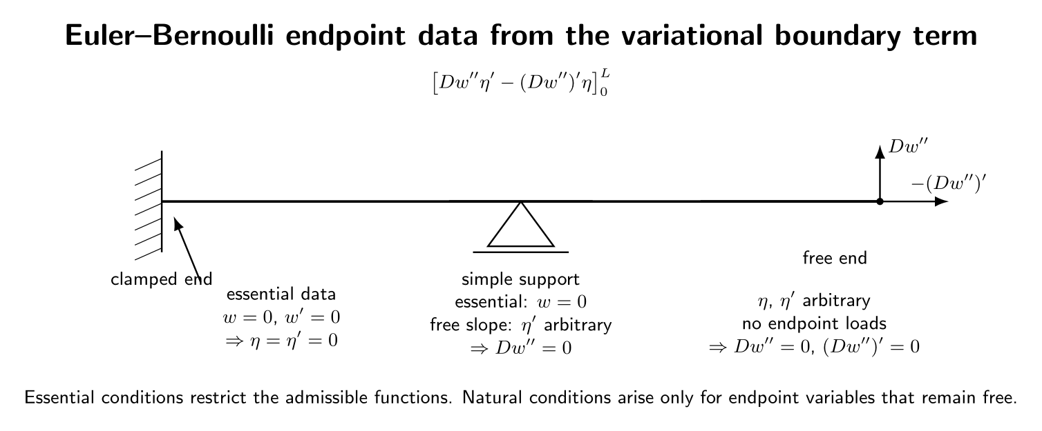
Figure. The beam problem exposes the two endpoint channels of a second-order
functional. Prescribed displacement and slope are essential data. When they are free, their
conjugate natural quantities are bending-moment-like and shear-like boundary terms.
1 Exercises
Exercise 1: derive the Euler–Bernoulli equation from total potential energy
Consider
- Compute the first variation δΠ[w; η].
- Integrate by parts twice and identify the interior equation.
- Identify the two natural boundary quantities conjugate to η and η′.
- Specialize the differential equation to constant EI.
Exercise 2: uniformly loaded cantilever
A beam of length L and constant flexural rigidity EI is clamped at x = 0 and free at x = L. It
carries a constant distributed load q > 0.
- State the essential conditions at the clamped end.
- Derive the natural conditions at the free end.
- Solve the beam equation for w(x).
- Find the free-end slope w′(L) and deflection w(L).
Exercise 3: uniformly loaded simply supported beam
A uniform beam has simple supports at x = 0 and x = L and carries the same constant load
q.
- Explain why w = 0 is essential at each support while the zero-moment condition is
natural.
- Solve for w(x).
- Find the maximum deflection and its location.
Exercise 4: clamped–clamped beam under uniform load
A uniform beam is clamped at both ends and carries constant q.
- State the four essential endpoint conditions.
- Solve for w(x).
- Compare the midspan deflection with the simply supported result from Exercise 3.
Exercise 5: cantilever with a concentrated tip force
A uniform cantilever has no distributed load. A force P > 0 acts at the free tip in the positive w
direction. Use
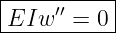
- Derive the differential equation and free-end natural conditions directly from δΠ = 0.
- Solve for w(x).
- Find the tip slope and tip deflection.
- Explain how the endpoint force appears through a boundary condition rather than
through the interior differential equation.
Exercise 6: variable flexural rigidity with a tip moment
A cantilever has
and a terminal moment M applied at x = L. There is no distributed load. Use
- Derive the free-end conditions.
- Show that the bending moment D(x)w′′(x) is constant.
- For α≠0, determine w′(x) and w(x) when w(0) = w′(0) = 0.
- Check the limit α → 0.
Exercise 7: endpoint springs and generalized natural conditions
A beam has no distributed load near its right end, but the endpoint is attached to a translational
spring of stiffness kt and a rotational spring of stiffness kr. An external tip force P also acts there.
The endpoint contribution to the potential is
For constant EI, derive the two natural conditions at x = L when both w(L) and w′(L) are
free.
Exercise 8: beam under axial tension
Consider the functional
- Derive the Euler–Lagrange equation.
- Derive the two natural boundary conditions at a completely free end.
- Explain physically why the quantity conjugate to endpoint displacement is no longer
simply −EIw′′′.
Exercise 9: one-parameter Rayleigh–Ritz estimate for a tip-loaded cantilever
Return to the cantilever of Exercise 5. Instead of solving the exact fourth-order boundary-value
problem, restrict the admissible set to
This trial family satisfies the clamped essential conditions but does not impose the free-end natural
conditions in advance.
- Substitute wa into the exact potential energy and find Π(a).
- Minimize with respect to a.
- Compute the Ritz estimate of the tip deflection.
- Compare with the exact result from Exercise 5.
- Explain why essential conditions must be built into a Ritz trial function but natural
conditions need not be.
2 Worked solutions
Solution 1: derive the Euler–Bernoulli equation from total potential energy
The integrand is
Therefore
The first variation is
Integrate the second term by parts once:
Integrate the remaining integral by parts again:
Hence
| δΠ | = ![[Dw ′′η′ − (Dw ′′)′η ]](https://images.physicslibrary.org/cache/objects/1206/make4ht/CalculusOfVariationsEulerBernoulliBeamProblemsAndWorkedSolutions14x.png) 0L
0L | (15)
|
| + ∫
0L![[(Dw ′′)′′ − q]](https://images.physicslibrary.org/cache/objects/1206/make4ht/CalculusOfVariationsEulerBernoulliBeamProblemsAndWorkedSolutions15x.png) η dx. η dx. | (16) |
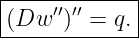
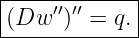
For arbitrary interior variations, the Fundamental Lemma gives
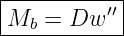
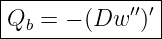
The two boundary quantities are therefore
as the quantity conjugate to the slope variation η′, and
as the quantity conjugate to the displacement variation η. The symbols Mb and Qb are deliberately
called moment-like and shear-like because detailed structural sign conventions differ. The
variational statement itself fixes their signs once the positive directions of w, q, endpoint force, and
endpoint moment have been chosen.
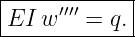
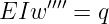
For constant EI,
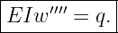
This is the static Euler–Bernoulli beam equation in the present sign convention [3, 2].
Solution 2: uniformly loaded cantilever
At the clamp,
These are essential conditions, so
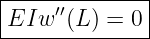
At the free end there is no applied endpoint moment or force. Both η(L) and η′(L) are arbitrary, so
the boundary term requires
Thus
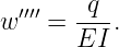
The differential equation is
Integrate four times:
| w′′′ | =  x + C1, x + C1, | (26)
|
| w′′ | =  x2 + C
1x + C2, x2 + C
1x + C2, | (27)
|
| w′ | =  x3 + x3 +  C1x2 + C
2x + C3, C1x2 + C
2x + C3, | (28)
|
| w | =  x4 + x4 +  C1x3 + C1x3 +  C2x2 + C
3x + C4. C2x2 + C
3x + C4. | (29) |
The free-end conditions give
while the clamped conditions give
Therefore
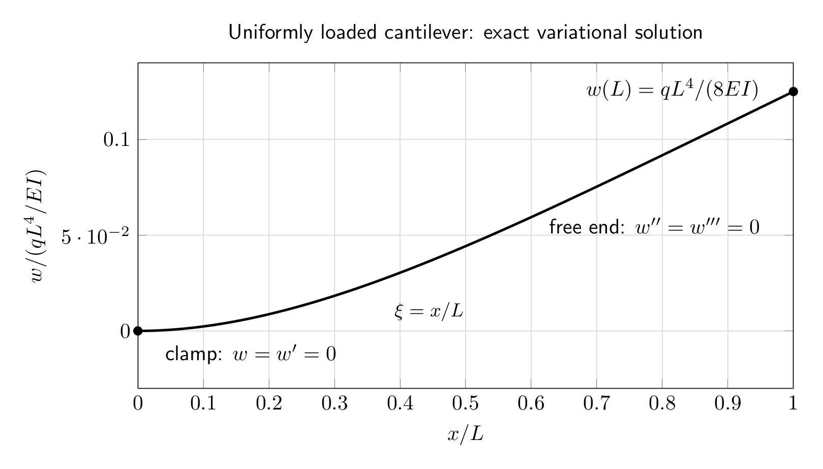
Figure. Normalized deflection of a uniformly loaded cantilever. The clamp enforces zero
displacement and slope; the free end satisfies zero natural bending moment and shear.
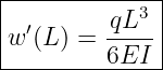
Differentiate:
At x = L,
and
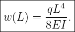
Solution 3: uniformly loaded simply supported beam
A simple support prevents transverse displacement but does not prescribe the slope.
Hence
are essential conditions, giving
The slope variations η′(0) and η′(L) remain free. Therefore the coefficients of those variations must
vanish:
Thus the zero bending moment at a simple support emerges as a natural boundary
condition.
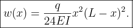
Solving
with
gives
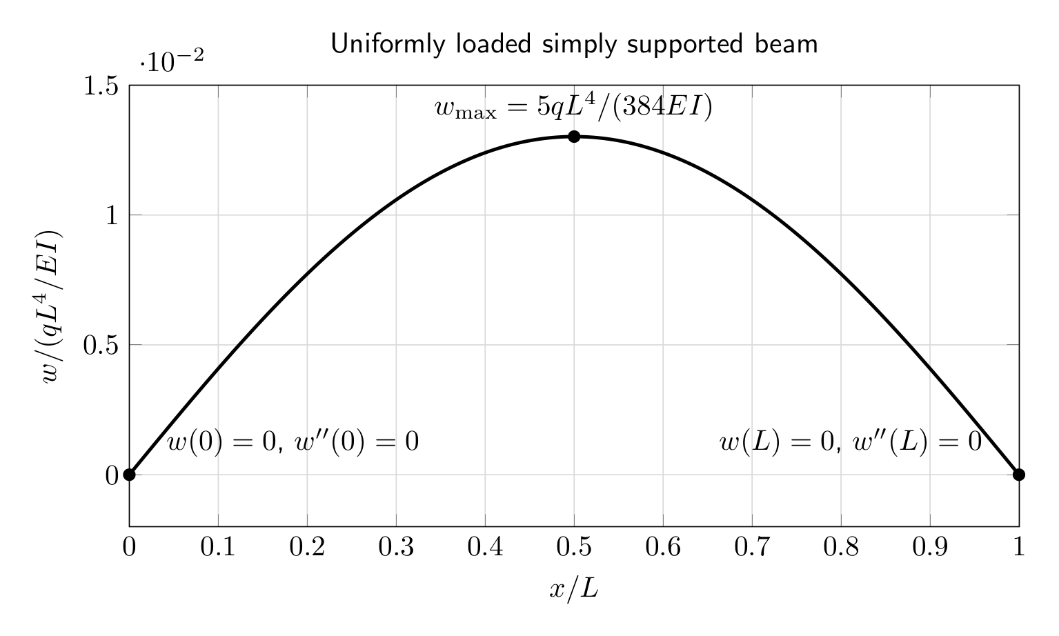
Figure. The simply supported beam has prescribed displacement at both ends but free
slope. Zero endpoint moment therefore arises naturally from stationarity.
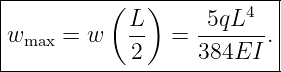
By symmetry, the maximum occurs at
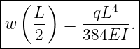
Substitution gives
Solution 4: clamped–clamped beam under uniform load
Both displacement and slope are prescribed at both ends:
All four endpoint variations therefore vanish. There are no natural conditions to derive because no
endpoint kinematic variable is free.
Solving EIw′′′′ = q gives
At midspan,
The simply supported maximum from Exercise 3 was
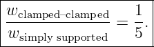
Thus the clamped–clamped midspan deflection is only one fifth as large:
The stronger kinematic restrictions make the beam substantially stiffer under the same
loading.
Solution 5: cantilever with a concentrated tip force
The potential is
Its variation is
After two integrations by parts,
| δΠ | = ![′′ ′ ′′′
[EIw η − EIw η]](https://images.physicslibrary.org/cache/objects/1206/make4ht/CalculusOfVariationsEulerBernoulliBeamProblemsAndWorkedSolutions53x.png) 0L
0L | (51)
|
| + ∫
0LEIw′′′′η dx − Pη(L). | (52) |
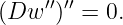
The clamped end removes the x = 0 terms. Since there is no distributed load,
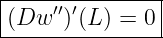
At the free end, η(L) and η′(L) are independent. Their coefficients give
and
Equivalently,
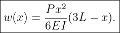
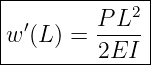
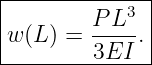
Solving with w(0) = w′(0) = 0 gives
Therefore
and
The key variational point is that the tip force is represented by the endpoint potential
−Pw(L). It therefore modifies the boundary equation but not the load-free interior equation
EIw′′′′ = 0.
Solution 6: variable flexural rigidity with a tip moment
Now
The first variation is
| δΠ | = ![[Dw ′′η′ − (Dw ′′)′η]](https://images.physicslibrary.org/cache/objects/1206/make4ht/CalculusOfVariationsEulerBernoulliBeamProblemsAndWorkedSolutions62x.png) 0L
0L | (61)
|
| + ∫
0L(Dw′′)′′η dx − Mη′(L). | (62) |
At the free end,
and
The interior equation is
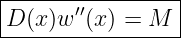
Hence Dw′′ is linear in x. The zero-shear condition says its derivative vanishes at L, so the linear
function is actually constant. The moment condition then gives
throughout the beam.
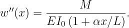
Therefore
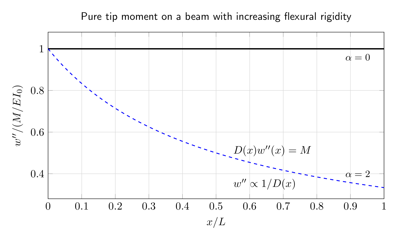
Figure. Under a pure terminal moment the internal bending moment is constant, but the
curvature is inversely proportional to the local flexural rigidity. A beam that becomes
stiffer toward the tip bends less there.
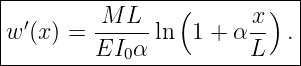
For α≠0, integrate once and use w′(0) = 0:
Integrate again and use w(0) = 0:
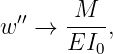
As α → 0,
so
which is the familiar constant-curvature result.
Solution 7: endpoint springs and generalized natural conditions
The beam contribution at x = L is
The endpoint potential contributes
Collect the coefficients of the independent endpoint variations.
For η′(L):
Thus
For η(L):
Hence
These are mixed, or Robin-type, natural boundary conditions. The endpoint springs interpolate
continuously between free and strongly restrained endpoint behavior.
Solution 8: beam under axial tension
The integrand is
Therefore
The second-order Euler–Lagrange equation is
For constant T and EI,
Thus
The boundary term is
At a completely free end with no endpoint loads,
and
The displacement-conjugate boundary quantity now contains both the bending contribution
−EIw′′′ and the transverse component associated with axial Tension, Tw′. This is exactly what
the variational boundary term predicts.
Solution 9: one-parameter Rayleigh–Ritz estimate for a tip-loaded cantilever
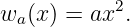
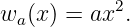
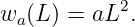
Choose
Then
and
Substitute into
| Π(a) | =  ∫
0LEI(2a)2dx − PaL2 ∫
0LEI(2a)2dx − PaL2 | (90)
|
| = 2EILa2 − PL2a. | (91) |
Stationarity in the one-dimensional trial space requires
Hence
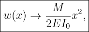
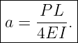
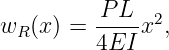
The Ritz approximation is therefore
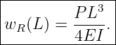
with tip deflection
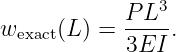
The exact result from Exercise 5 is
Thus
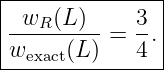
The one-parameter approximation underestimates the compliance by 25%.
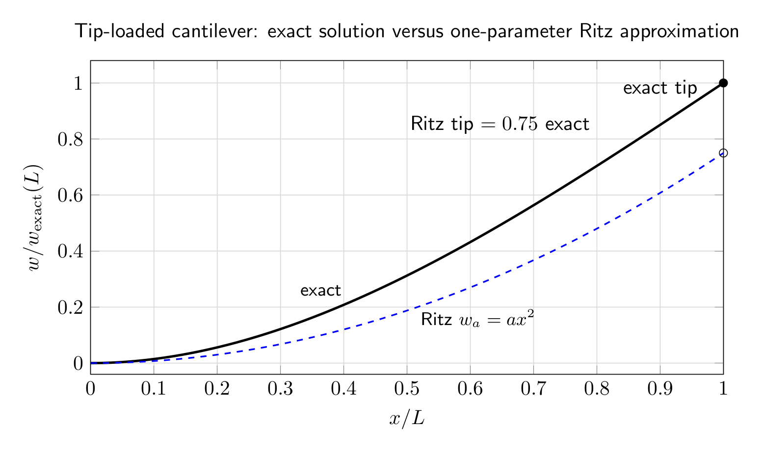
Figure. Exact and one-parameter Rayleigh–Ritz cantilever shapes, normalized by the
exact tip deflection. The Ritz curve satisfies the clamped essential conditions but is not
forced to satisfy the free-end moment condition beforehand.
This last point is fundamental. Essential boundary conditions define the admissible function space,
so every trial function must satisfy them. Natural boundary conditions arise from stationarity of
the functional itself. A Ritz approximation should therefore be allowed to discover them only
approximately through energy minimization rather than impose them as artificial kinematic
restrictions [2].
3 What the beam examples teach about higher-order variational problems
The beam equations make several abstract points from CV08 concrete.
- A functional depending on w′′ naturally produces a fourth-order differential equation.
- The endpoint variables w and w′ are independent kinematic channels.
- Their conjugate boundary quantities arise directly from repeated integration by parts.
- Loads can enter either through the interior functional, as q(x) does, or through endpoint
potentials, as P and M do.
- A boundary condition is not “essential” or “natural” because of its physical name; the
distinction is variational. Essential data are imposed on the admissible class. Natural
data emerge from free endpoint variations.
- Variable stiffness is handled without changing the variational principle: one simply
retains derivatives of D(x)w′′ rather than replacing them prematurely by EIw′′′′.
- Rayleigh–Ritz methods are finite-dimensional restrictions of the same energy principle.
4 Common mistakes
- Replacing (Dw′′)′′ by Dw′′′′ when D varies with x. That simplification is valid
only for constant flexural rigidity.
- Imposing zero slope at a simple support. A simple support fixes displacement
but ordinarily leaves rotation free.
- Imposing w′′ = w′′′ = 0 at every endpoint. Those are free-end natural conditions
for a uniform beam with no endpoint loads, not universal beam conditions.
- Forgetting endpoint work. A tip force or moment changes the natural boundary
condition even when the interior loading is zero.
- Using the wrong sign convention for shear or moment without declaring
it. The variational derivation is internally consistent, but engineering sign conventions
differ across texts.
- Building natural conditions into every Ritz trial function. Trial functions must
satisfy essential conditions; natural conditions generally follow from stationarity.
- Assuming Euler–Bernoulli theory is exact for every beam. Short, thick
beams or cases with important transverse shear require more refined theories such as
Timoshenko beam theory.
Summary
For the Euler–Bernoulli potential
stationarity gives
For constant rigidity,
The associated boundary term is
This compact expression contains the essential/natural boundary-condition logic for
clamped, simply supported, free, elastically restrained, force-loaded, and moment-loaded
endpoints. It is one of the most useful physical examples of the higher-order calculus of
variations.
References
[1] I. M. Gelfand and S. V. Fomin, Calculus of Variations, Dover Publications, 2000.
[2] J. N. Reddy, Energy Principles and Variational Methods in Applied Mechanics, 2nd
ed., John Wiley & Sons, 2002.
[3] S. P. Timoshenko and J. M. Gere, Mechanics of Materials, Van Nostrand Reinhold,
1972.
[4] L. D. Landau and E. M. Lifshitz, Theory of Elasticity, 3rd ed.,
Butterworth-Heinemann, 1986.
[5] Cornelius Lanczos, The Variational Principles of Mechanics, 4th ed., Dover
Publications, 1986.

![[parent]](https://images.physicslibrary.org/images/uparrow.png)

![∫ [ ]
L 1- ′′ 2
Π [w ] = 2D (x) w (x) − q(x)w (x ) dx + endpoint potential terms.
0](https://images.physicslibrary.org/cache/objects/1206/make4ht/CalculusOfVariationsEulerBernoulliBeamProblemsAndWorkedSolutions1x.png)
![∫ L[ 1 ]
Π[w ] = -D (x)w ′′2 − q(x)w dx.
0 2](https://images.physicslibrary.org/cache/objects/1206/make4ht/CalculusOfVariationsEulerBernoulliBeamProblemsAndWorkedSolutions2x.png)
![1 ∫ L
Π [w ] = -- EI w′′2 dx − P w(L ).
2 0](https://images.physicslibrary.org/cache/objects/1206/make4ht/CalculusOfVariationsEulerBernoulliBeamProblemsAndWorkedSolutions3x.png)

![∫
1- L ′′2 ′
Π[w ] = 2 D (x)w dx − M w (L).
0](https://images.physicslibrary.org/cache/objects/1206/make4ht/CalculusOfVariationsEulerBernoulliBeamProblemsAndWorkedSolutions5x.png)

![∫ L [ ]
1- ′′2 1- ′2
Π [w] = 0 2EI w + 2 T w − q(x )w dx, T > 0.](https://images.physicslibrary.org/cache/objects/1206/make4ht/CalculusOfVariationsEulerBernoulliBeamProblemsAndWorkedSolutions7x.png)


![∫ L
δΠ = [− qη + Dw ′′η′′]dx.
0](https://images.physicslibrary.org/cache/objects/1206/make4ht/CalculusOfVariationsEulerBernoulliBeamProblemsAndWorkedSolutions11x.png)
![∫ ∫
L ′′ ′′ ′′ ′L L ′′ ′′
Dw η dx = [Dw η ]0 − (Dw )η dx.
0 0](https://images.physicslibrary.org/cache/objects/1206/make4ht/CalculusOfVariationsEulerBernoulliBeamProblemsAndWorkedSolutions12x.png)
![∫ L ∫ L
− (Dw ′′)′η′dx = − [(Dw ′′)′η]L+ (Dw ′′)′′ηdx.
0 0 0](https://images.physicslibrary.org/cache/objects/1206/make4ht/CalculusOfVariationsEulerBernoulliBeamProblemsAndWorkedSolutions13x.png)
















![∫
1- L ′′2
Π [w] = 2 EI w dx − Pw (L).
0](https://images.physicslibrary.org/cache/objects/1206/make4ht/CalculusOfVariationsEulerBernoulliBeamProblemsAndWorkedSolutions51x.png)




![1∫ L
Π [w ] = -- D (x)w ′′2dx − M w ′(L ).
2 0](https://images.physicslibrary.org/cache/objects/1206/make4ht/CalculusOfVariationsEulerBernoulliBeamProblemsAndWorkedSolutions61x.png)

![|-------------2-[(-------)---(--------)---(--------)----]--|
|w (x) = -M-L--- 1 + α x- ln 1 + αx- − 1 + α x + 1 .|
---------EI0-α2---------L-----------L------------L---------|](https://images.physicslibrary.org/cache/objects/1206/make4ht/CalculusOfVariationsEulerBernoulliBeamProblemsAndWorkedSolutions69x.png)

![′ ′
δΦ = [ktw (L) − P ]η(L) + krw (L )η (L ).](https://images.physicslibrary.org/cache/objects/1206/make4ht/CalculusOfVariationsEulerBernoulliBeamProblemsAndWorkedSolutions73x.png)









![[(T w ′ − EIw ′′′)η + EIw ′′η′]L .
0](https://images.physicslibrary.org/cache/objects/1206/make4ht/CalculusOfVariationsEulerBernoulliBeamProblemsAndWorkedSolutions83x.png)


![∫
1 L ′′2
Π [w ] = -- EIw dx − P w (L ) :
2 0](https://images.physicslibrary.org/cache/objects/1206/make4ht/CalculusOfVariationsEulerBernoulliBeamProblemsAndWorkedSolutions89x.png)

![∫ [ ]
L 1- ′′2
Π[w ] = 2D (x)w − q(x)w dx,
0](https://images.physicslibrary.org/cache/objects/1206/make4ht/CalculusOfVariationsEulerBernoulliBeamProblemsAndWorkedSolutions97x.png)
![|----′′-′------′′′--L-|
[Dw---η-−-(Dw--)-η]0 .-](https://images.physicslibrary.org/cache/objects/1206/make4ht/CalculusOfVariationsEulerBernoulliBeamProblemsAndWorkedSolutions100x.png)