Wave Mechanics: Energy in a 1D Wave
The previous articles developed the one-dimensional string wave equation,
and its traveling-wave solutions. The string does more than move, however. A disturbance also
carries mechanical energy.
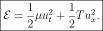
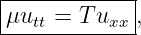
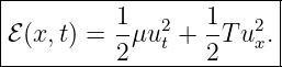
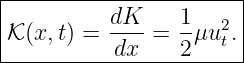
For the ideal stretched string, the local mechanical energy per unit equilibrium length
is
The first term is kinetic energy density and the second is elastic potential energy density. This
expression is standard for transverse waves on an ideal stretched string and follows directly from
the same small-slope model used to derive the wave equation [1, 2, 3, 5].
WM18 develops that result from the mechanics of a short string element, checks its dimensions,
applies it to traveling waves and Standing Waves, and shows why wave energy scales as the square
of amplitude. The next article will ask how this energy crosses a fixed position and will derive the
corresponding power flow.
1 Energy is distributed along the string
A string is a continuous system. Rather than assigning one energy to one point, we describe the
energy contained in a short equilibrium-length interval dx.
Write
where ℰ has units of energy per unit length.
For an ideal string there are two mechanical contributions:
The local bookkeeping is summarized below.

Figure. A moving string element has kinetic energy through ut. A sloped element is
slightly longer than its equilibrium projection dx, producing elastic potential energy
through ux.
2 Kinetic energy density
Consider a short string element of equilibrium length dx. Its mass is
where μ is the linear mass density.
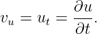
The transverse velocity of the material point at position x is
Therefore the kinetic energy of the element is
| dK | =  dmvu2 dmvu2 | (7)
|
| =  (μdx)ut2. (μdx)ut2. | (8) |
Divide by dx:
This expression is exact within the transverse-motion model used here: kinetic energy is controlled
by the local material velocity, not by the propagation speed alone.
3 Elastic potential energy density
The potential-energy term requires the string geometry.
At a fixed time, a short displaced string element has arclength
Since
we obtain
For the small-slope model,
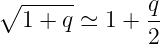
Use the expansion
for small q. With q = ux2,
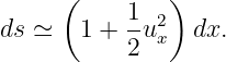
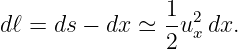
The extra length is therefore
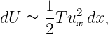
If the equilibrium Tension magnitude is approximately constant at T, the work required to create
this additional length is
Thus
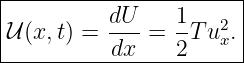
and the elastic potential energy density is
The same small-slope approximation that linearized the force law in WM14 also gives this
quadratic elastic-energy expression.
4 Total local energy density
Adding the kinetic and potential terms gives
This formula contains an important physical separation:
- ut measures how rapidly the material is moving through equilibrium space;
- ux measures how much the string is locally tilted and therefore stretched relative to
its equilibrium projection.
A point can have zero displacement while still carrying energy. Energy depends on velocity and
deformation, not simply on the value of u.
5 Dimensional check
The kinetic term has dimensions
For the potential term, ux is dimensionless because both u and x have dimensions of length.
Hence
Both terms therefore have the required units of energy per unit length.
6 Pure traveling waves have equal kinetic and potential densities
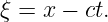
Consider a right-moving traveling profile
Let
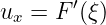
Then
and
The kinetic energy density becomes
For the ideal string,
so
Therefore
But
Hence
for every point of a pure right-moving wave. The same proof holds for a pure left-moving wave
G(x + ct).
The total energy density of a pure traveling wave can therefore be written as
A pulse example is shown below.
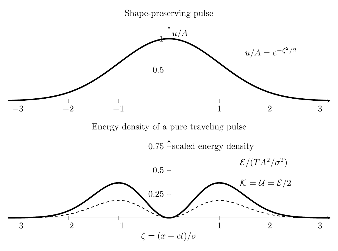
Figure. For a Gaussian pure traveling pulse, with normalized coordinate ζ = (x − ct)∕σ,
the kinetic and elastic potential energy densities are equal point by point. The energy
density depends on the square of the pulse slope, so a smooth pulse can have zero energy
density exactly at its displacement maximum.
7 Why the center of a smooth pulse can have zero energy density
This result can initially seem surprising. Consider a smooth pulse at its maximum. At the exact
peak,
For a shape-preserving traveling pulse,
and
Therefore both local energy-density terms vanish at the exact pulse peak.
The pulse still carries finite total energy because energy is distributed over the regions
where the profile changes. Large displacement alone is not the same as large local wave
energy.
8 Sinusoidal traveling wave
Consider
Define
Then
and
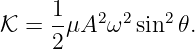
The kinetic energy density is
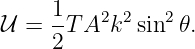
The potential energy density is
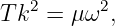
The ideal-string dispersion relation is
with
Thus
so again
The total energy density is

Figure. The displacement varies as cos 𝜃, while the energy density varies as sin 2𝜃. Energy
density is nonnegative and repeats twice during one displacement phase cycle.
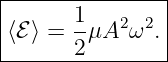
9 Average energy density of a sinusoidal traveling wave
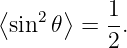
Over one full phase cycle,
Therefore
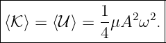
The average kinetic and average potential contributions are each half of this:
The energy contained in one wavelength, averaged over the sinusoidal phase pattern,
is
Hence
This result agrees with standard treatments of sinusoidal mechanical waves [3].
10 Energy scales as amplitude squared and frequency squared
For fixed μ, the average sinusoidal energy density obeys
Therefore:
- doubling the amplitude multiplies average energy density by 4;
- tripling the angular frequency at fixed amplitude multiplies it by 9;
- changing the sign of the displacement amplitude does not change the energy.
This square-law behavior is one of the most important recurring features of wave physics.
Similar quadratic energy measures will appear later for acoustic, electromagnetic, and
quantum-wave contexts, although the detailed physical meaning of the field variables
changes.
11 A general two-direction field
WM16 showed that a sufficiently smooth whole-line solution can be written as
Let
Then
and
Use T = μc2. The total energy density is
| ℰ | =  μc2[−F′ + G′]2 + μc2[−F′ + G′]2 +  T[F′ + G′]2 T[F′ + G′]2 | (58)
|
| =  [−F′ + G′]2 + [−F′ + G′]2 +  [F′ + G′]2. [F′ + G′]2. | (59) |
Expanding the squares, the cross terms cancel:
This is a useful result. The displacement fields interfere linearly, but in the ideal string model the
total mechanical energy density separates into the sum of the directional component energy
densities.
The kinetic and potential parts individually need not be equal when both directions are
present.
12 Standing waves exchange kinetic and potential energy
A standing wave can be written
with fixed ends chosen so that
The derivatives are
and
Thus
and
Unlike a single traveling wave, these two densities are not generally equal point by point.
Integrating over a normal-mode length 0 ≤ x ≤ L gives
and
Therefore
which is constant in the ideal lossless model.
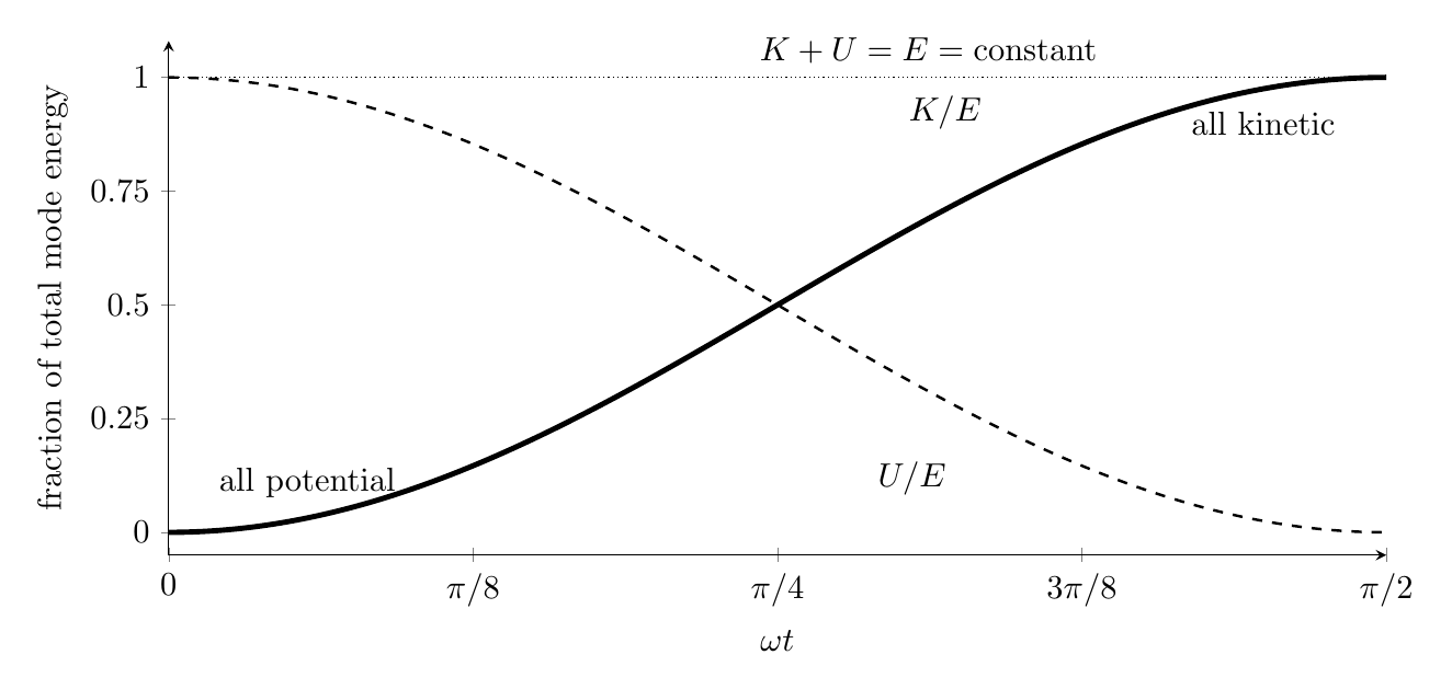
Figure. For one ideal standing-wave normal mode, total energy is constant while the
integrated kinetic and elastic potential energies exchange periodically.
13 Worked Example 1: Local energy density from measured slope and velocity
A string has
At one event (x,t), suppose
and
Find the kinetic, potential, and total energy densities.
Solution
The kinetic density is
| 𝒦 | =  μut2 μut2 | (73)
|
| =  (0.020)(1.5)2 (0.020)(1.5)2 | (74)
|
| = 0.0225 J/m. | (75) |
The potential density is
| 𝒰 | =  Tux2 Tux2 | (76)
|
| =  (80)(0.080)2 (80)(0.080)2 | (77)
|
| = 0.256 J/m. | (78) |
Therefore
The kinetic and potential densities are not equal here. Equality is guaranteed point by point only
for a pure traveling wave moving at the string wave speed.
14 Worked Example 2: Sinusoidal average energy density and energy per wavelength
A sinusoidal traveling wave has
on a string with
Find the wave speed, wavelength, average energy density, and average energy contained in one
wavelength.
Solution
First convert the amplitude:
The wave speed is
| c | =  | (83)
|
| =  | (84)
|
| = 79.1 m/s. | (85) |
The wavelength is
| λ | =  | (86)
|
| =  | (87)
|
| = 1.58 m. | (88) |
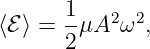
The angular frequency is
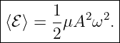
The average energy density is
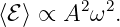
| ⟨ℰ⟩ | =  μA2ω2 μA2ω2 | (90)
|
| =  (0.012)(0.0040)2(314.2)2 (0.012)(0.0040)2(314.2)2 | (91)
|
| ≃ 9.47 × 10⁻³ J/m. | (92) |
Thus
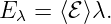
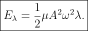
The energy per wavelength is
| Eλ | = ⟨ℰ⟩λ | (94)
|
| = (9.47 × 10⁻³)(1.58) | (95)
|
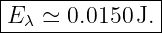
| ≃ 1.50 × 10⁻² J. | (96) |
Therefore
15 Worked Example 3: Total energy of a Gaussian traveling pulse
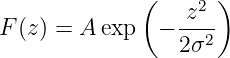
Consider the right-moving pulse
Let
Find the total mechanical energy of the pulse.
Solution
Let
Then
and
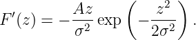
For a pure traveling wave,
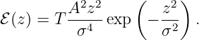
Hence
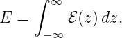
The total energy is
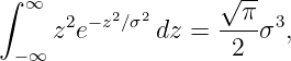
Using
we obtain
Now use
Then
| E | = 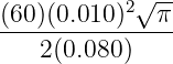 | (110)
|
| ≃ 6.65 × 10⁻² J. | (111) |
Therefore
The result scales as A2 and inversely with the pulse width parameter σ: for the same peak
displacement, a sharper pulse has larger slopes and therefore more energy.
16 Worked Example 4: Amplitude and frequency scaling
Wave 1 and wave 2 travel on the same string. Suppose
and
Find the ratio of their average sinusoidal energy densities.
Solution
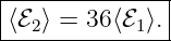
Since
and both waves are on the same string,
 | =  | (116)
|
| = (2)2(3)2 | (117)
|
| = 36. | (118) |
Thus
The square-law scaling compounds rapidly when both amplitude and frequency increase.
17 Worked Example 5: Energy exchange in a standing mode
A fixed-fixed string normal mode is
with
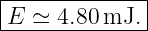
Find the total mode energy, and find the integrated kinetic and potential energies when
Solution
Convert the amplitude:
The angular frequency is
The constant total mode energy is
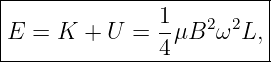
| E | =  μB2ω2L μB2ω2L | (125)
|
| =  (0.015)(0.0060)2(188.5)2(1.0) (0.015)(0.0060)2(188.5)2(1.0) | (126)
|
| ≃ 4.80 × 10⁻³ J. | (127) |
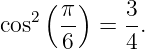
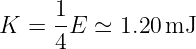
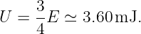
Therefore
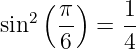
At ωt = π∕6,
and
Hence
and
So
Their sum remains the same total mechanical energy.
18 Worked Example 6: Energy density of simultaneous right- and left-moving components
At one event, suppose a two-direction solution has
Find the total energy density. Also find the kinetic and potential parts separately.
Solution
For the two-family solution,
Therefore
| ℰ | = 50[(0.10)2 + (−0.040)2] | (136)
|
| = 50(0.0116) | (137)
|
| = 0.580 J/m . | (138) |
For the kinetic part,
Using μc2 = T,
| 𝒦 | =  (−F′ + G′)2 (−F′ + G′)2 | (140)
|
| =  (−0.10 − 0.040)2 (−0.10 − 0.040)2 | (141)
|
| = 25(0.0196) | (142)
|
| = 0.490 J/m . | (143) |
For the potential part,
| 𝒰 | =  (F′ + G′)2 (F′ + G′)2 | (144)
|
| = 25(0.10 − 0.040)2 | (145)
|
| = 25(0.0036) | (146)
|
| = 0.0900 J/m . | (147) |
As a check,
The kinetic and potential densities are not equal because this field contains both propagation
directions at once.
19 Common mistakes
- Mistake: treating displacement amplitude itself as energy. Energy depends on squared
velocity and squared slope.
- Mistake: using the propagation speed c in place of the material velocity ut in the
kinetic energy.
- Mistake: assuming 𝒦 = 𝒰 for every wave field. Pointwise equality holds for a pure
traveling wave, not for an arbitrary superposition or standing wave.
- Mistake: forgetting that ux is dimensionless for transverse displacement u measured
in meters against coordinate x measured in meters.
- Mistake: assuming the displacement maximum of a pulse must also be the local
energy-density maximum. For a smooth pure traveling pulse, the exact displacement
peak can have zero slope and zero transverse velocity.
- Mistake: applying the ideal-string energy density outside the small-slope,
constant-tension model without checking whether the approximations remain valid.
20 What WM18 establishes
The ideal one-dimensional string contains mechanical energy with local density
For a pure traveling wave,
and, for a sinusoidal traveling wave,
The next question is no longer how much energy is locally present, but how rapidly
that energy passes a fixed position. That leads naturally to wave power and energy
flux.
References
References
[1] A. P. French, Vibrations and Waves, M.I.T. Introductory Physics Series, W. W.
Norton & Company, 1971.
[2] Frank S. Crawford, Jr., Waves, Berkeley Physics Course, Volume 3, McGraw-Hill,
1968.
[3] William Moebs, Samuel J. Ling, and Jeff Sanny, University Physics, Volume 1,
OpenStax, 2016, Section 16.4, “Energy and Power of a Wave.”
[4] Howard Georgi, The Physics of Waves, Benjamin/Cummings, 1992, continuum and
traveling-wave chapters; also distributed through MIT OpenCourseWare 8.03SC.
[5] Massachusetts Institute of Technology, 8.03SC Physics III: Vibrations and Waves,
Fall 2016, Problem Set 5 and Lecture 10 materials on traveling waves and string energy,
MIT OpenCourseWare.










![2
[μu2 ] = kg-m--= J-.
t m s2 m](https://images.physicslibrary.org/cache/objects/1183/make4ht/WaveMechanicsEnergyInA1DWave20x.png)
![J
[T u2x] = N = --.
m](https://images.physicslibrary.org/cache/objects/1183/make4ht/WaveMechanicsEnergyInA1DWave21x.png)


![𝒦 = 1μc2[F ′(ξ)]2.
2](https://images.physicslibrary.org/cache/objects/1183/make4ht/WaveMechanicsEnergyInA1DWave26x.png)


![1
𝒦 = -T [F ′(ξ )]2.
2](https://images.physicslibrary.org/cache/objects/1183/make4ht/WaveMechanicsEnergyInA1DWave29x.png)
![𝒰 = 1-Tu2x = 1T [F ′(ξ)]2.
2 2](https://images.physicslibrary.org/cache/objects/1183/make4ht/WaveMechanicsEnergyInA1DWave30x.png)

![|--------------------------------------|
|ℰ = T[F ′(x − ct)]2 = μc2[F ′(x − ct)]2. |
---------------------------------------](https://images.physicslibrary.org/cache/objects/1183/make4ht/WaveMechanicsEnergyInA1DWave32x.png)















![|--------------------------|
|ℰ = T [F ′(ξ)]2 + T[G ′(η)]2.|
---------------------------](https://images.physicslibrary.org/cache/objects/1183/make4ht/WaveMechanicsEnergyInA1DWave61x.png)

















![[ 2]
u(x,t) = A exp − (x-−-ct)- .
2σ2](https://images.physicslibrary.org/cache/objects/1183/make4ht/WaveMechanicsEnergyInA1DWave91x.png)


![ℰ = T [F ′(z )]2.](https://images.physicslibrary.org/cache/objects/1183/make4ht/WaveMechanicsEnergyInA1DWave96x.png)













![ℰ = T[(F ′)2 + (G′)2].](https://images.physicslibrary.org/cache/objects/1183/make4ht/WaveMechanicsEnergyInA1DWave126x.png)