|
|
|
|||||||
so an outward wave carries the radial phase factor e−ikr. For a z-directed Hertzian element with current moment I0ℓ in a lossless medium,
and
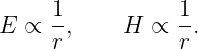
In the radiation zone,
with
For the ideal Hertzian element,
and in free space
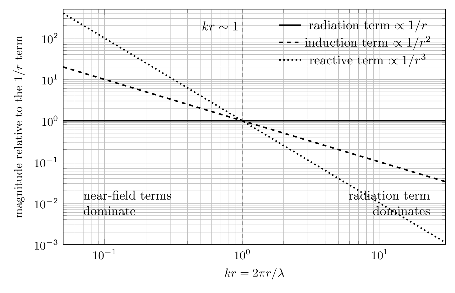
Figure. Relative magnitudes of the induction and reactive terms when the 1∕r radiation term is used as the reference. The controlling dimensionless distance is kr = 2πr∕λ.
How to use this problem setAttempt all problems in Part I before consulting Part II. For numerical problems in vacuum, use
Keep a clear distinction among field amplitude, power density, radiation intensity, total power, and radiation resistance.
Part I: Exercises
Exercise 1: retarded time and propagation phaseA sinusoidal source operates at
An observation point is one quarter wavelength from the source in vacuum.
Exercise 2: is the element electrically short?A straight current element has physical length
Evaluate ℓ∕λ at 1.00 GHz and 10.0 GHz. Discuss at which frequency the ideal Hertzian approximation is more credible and why the condition ℓ ≪ λ matters.
Exercise 3: comparing the 1∕r, 1∕r2, and 1∕r3 termsInside E𝜃, compare the magnitudes of the induction and reactive terms with the radiation term. Show that
and
Evaluate both ratios for
Interpret the trend physically.
Exercise 4: exact Hertzian-dipole fields in the transition regionIn vacuum let
At
calculate the complex phasors Er, E𝜃, and Hϕ. Report magnitudes and phases. Explain why the simple far-field relation E∕H = η0 should not yet be expected for the total local fields.
Exercise 5: exact field versus far-field approximationUse the same 300 MHz Hertzian element as Exercise 4, but evaluate the broadside field at
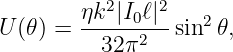
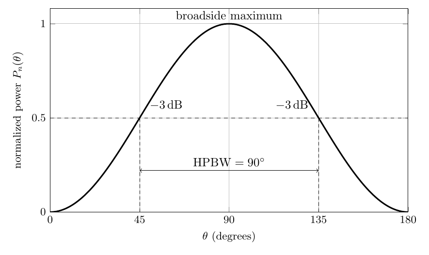
Exercise 6: radiation pattern and half-power beamwidthFor a Hertzian dipole,
Find the directions of the nulls, the direction of maximum radiation, the two half-power angles in the principal plane, and the half-power beamwidth.
Figure. The normalized Hertzian-dipole power pattern in a principal plane.
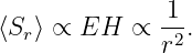
Exercise 7: power density and radiation intensityFor the 300 MHz element of Exercise 4, evaluate the far-field time-average power density and radiation intensity at
Verify that the radiation intensity is independent of r in the far field.
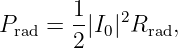
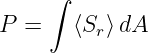
Exercise 8: derive the total radiated powerStarting from
with
derive the total power by integrating over solid angle:
Show every integration step and recover the EM23 result.
Figure. Total radiated power is obtained by integrating the outward far-field Poynting flux over a sphere.
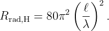
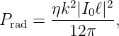
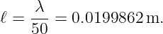
Exercise 9: radiated power and radiation resistanceFor the 300 MHz element with I0 = 1.00 A and ℓ = λ∕50:
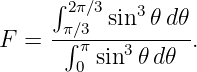
Exercise 10: what fraction of the power lies near broadside?Find the fraction of the total Hertzian-dipole radiated power that leaves through the angular band
The band includes all azimuth angles 0 ≤ ϕ < 2π.
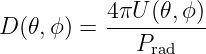
Exercise 11: derive directivity from the patternUse
to derive the maximum directivity of a Hertzian dipole. Express the result as a dimensionless ratio and in dBi.
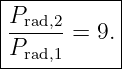
Exercise 12: frequency scaling at fixed physical lengthA physically fixed Hertzian current element is driven with the same current amplitude at 100 MHz and 300 MHz. Assume its length remains electrically short at both frequencies.
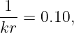
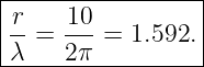
Exercise 13: distance required for small nonradiative termsFor the E𝜃 expression, determine the electrical distance kr and physical distance in wavelengths required so that
Explain why the boundary of the “far field” is not a single universal radius for every source and every accuracy requirement.
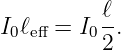
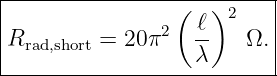
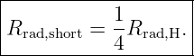
Exercise 14: Hertzian element versus a physically short dipoleA Hertzian element assumes uniform current along its infinitesimal length. A physically short center-fed dipole of total length ℓ is more realistically approximated by a triangular current distribution that falls from I0 at the feed to zero at the ends. If the triangular distribution has effective current moment I0ℓ∕2, use the Hertzian result to derive the radiation resistance of the physically short dipole. Compare it with the uniform-current Hertzian value for the same total length and feed current.
Exercise 15: spherical spreading and conservation of radiated powerAt a fixed far-field angle, show that the Hertzian-dipole power density satisfies
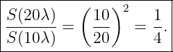
Compare the power density at r = 10λ and r = 20λ. Then explain why the total power through a sphere remains constant even though the local power density decreases.
Exercise 16: Julia sweep of field zones and radiation patternWrite a Julia program that:
State the numerical checks the program should reproduce.
Part II: Complete Worked Solutions
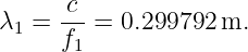
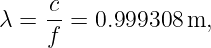
Solution 1: retarded time and propagation phaseThe wavelength is
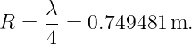
One quarter wavelength is
The propagation delay is
Thus
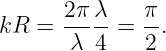
The Wavenumber is
so
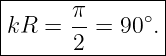
Therefore
In time language, the observation point sees the source 2.50 ns late. In phasor language, that same delay multiplies the source amplitude by
The delay and phase shift are two representations of the same finite propagation time.
Solution 2: is the element electrically short?At 1.00 GHz,
Hence
At 10.0 GHz,
so
Thus the element is much more plausibly approximated as electrically short at 1 GHz. At 10 GHz its length is about one third wavelength, so phase and current variation along the Conductor can no longer be ignored. The requirement ℓ ≪ λ allows the source current to be treated as nearly in phase over the entire element and permits the current distribution to be collapsed into the single current moment I0ℓ.
Solution 3: comparing the three radial familiesThe radiation contribution inside the E𝜃 bracket has magnitude proportional to
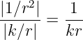
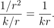
The induction contribution has magnitude 1∕r2, so
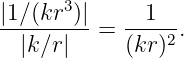
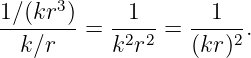
The reactive contribution has magnitude 1∕(kr3), giving
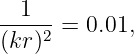
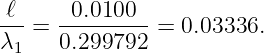
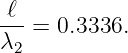
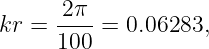
For r = λ∕100,
so
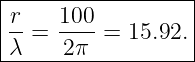
For r = λ∕(2π),
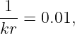
and both ratios equal unity. For r = λ,
so
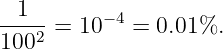
For r = 10λ,
so
The faster-decaying 1∕r2 and 1∕r3 contributions dominate close to the source but become negligible compared with the 1∕r radiation term as kr grows.
Solution 4: exact fields in the transition regionAt 300 MHz,
and
The observation radius is
so
Also,
Substituting into the complete field expressions gives
and
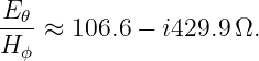
The ratio of the transverse fields is therefore complex:
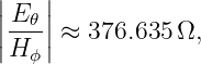
Its magnitude is not η0. This is expected because kr < 1 and the local field still contains strong induction and reactive contributions. The plane-wave-like ratio E∕H = η0 applies to the surviving radiation terms in the far zone, not to the complete transition-region field.
Solution 5: exact field versus far-field approximationAt broadside, sin 𝜃 = 1 and Er = 0. At
we have
Using the complete formulas gives
and
The far-field expression gives
The percentage amplitude error is
Thus the far-field approximation is already very accurate at 10λ for this ideal element. The exact transverse ratio is
which is extremely close to
Solution 6: radiation pattern and half-power beamwidthThe power pattern is
Nulls occur where
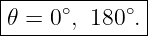
so
The maximum occurs at
Half power means
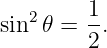
Therefore
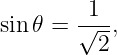
which gives
Hence the half-power beamwidth in that principal plane is
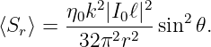
Solution 7: power density and radiation intensityThe far-field power density is
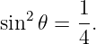
For 𝜃 = 30∘,
At r = 10λ the numerical result is
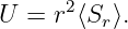
Radiation intensity is defined by
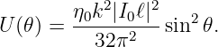
Hence
Because the far-field power density contains 1∕r2, multiplying by r2 removes the radial dependence:
Thus radiation intensity records angular power flow without depending on which far-field sphere is used.
Solution 8: total radiated powerStart with
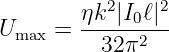
Since Umax is constant,
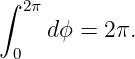
The azimuth integral is
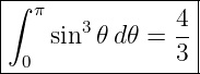
For the polar integral, write
Let
Then
Therefore
Substituting
gives
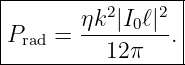
Solution 9: radiated power and radiation resistanceFor the numerical example,
Thus
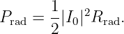
Radiation resistance is defined by
For I0 = 1 A,
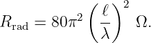
The closed-form formula gives
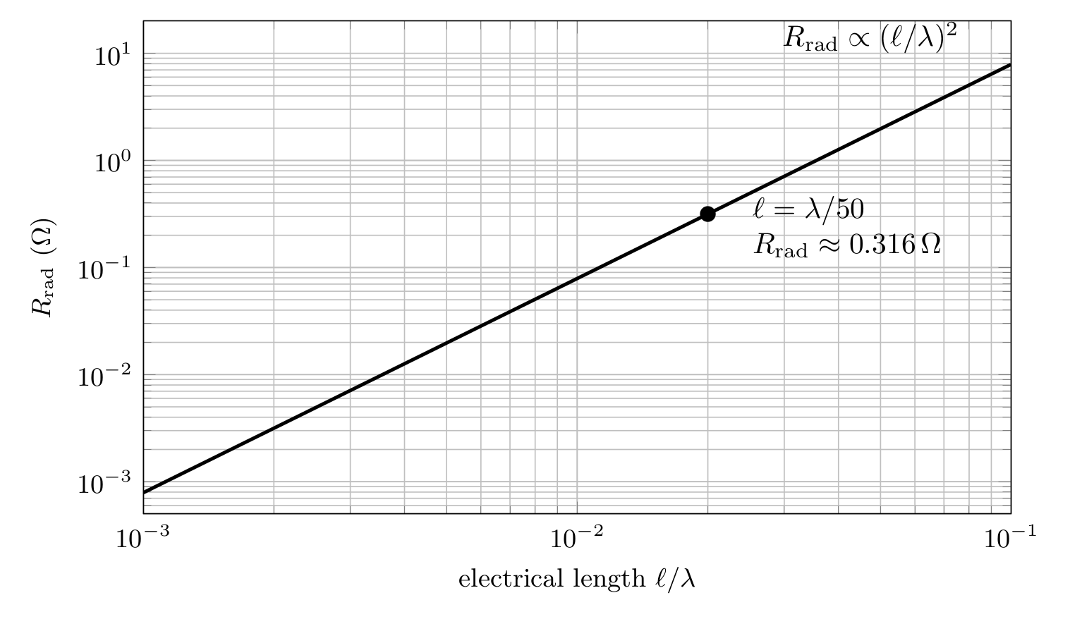
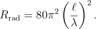
The familiar coefficient 80π2 uses the standard approximation η 0 ≈ 120π Ω. Using η0 = 376.7303 Ω directly gives 0.31561 Ω; using 120π Ω gives 0.31583 Ω. The distinction is only about 0.07% and does not change the antenna physics.
Figure. Hertzian-element radiation resistance rises quadratically with electrical length.
Solution 10: fraction of power near broadsideBecause all azimuth angles are included, the required fraction is
The denominator is 4∕3. An antiderivative is
Therefore
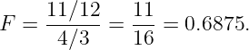
Hence
Thus
of the Hertzian-dipole power lies between 60∘ and 120∘.
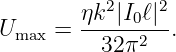
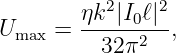
Solution 11: directivityThe maximum radiation intensity occurs at 𝜃 = 90∘:
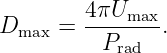
Directivity is
Substituting the expressions for Umax and Prad,
Therefore
In dBi,
Solution 12: frequency scaling at fixed physical lengthFor fixed physical length ℓ,
Since
we have
Increasing frequency from 100 to 300 MHz multiplies frequency by three, so
For unchanged current amplitude,
so
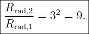
The physical element becomes electrically longer at higher frequency, making it a more effective radiator as long as the Hertzian approximation remains valid.
Solution 13: distance required for small nonradiative termsThe induction-to-radiation ratio is
For a 10% induction term,
so
Since
we obtain
At the same distance, the reactive-to-radiation ratio is
or 1%. For a 1% induction term,
so
and
At that distance the reactive ratio is
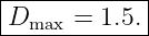
These estimates concern the ideal Hertzian field terms. A real finite antenna also has an aperture-size far-field criterion such as r ≳ 2D2∕λ, and the acceptable error depends on the application. Therefore there is no single universal far-field radius that applies to every radiator and accuracy requirement.
Solution 14: Hertzian element versus a physically short dipoleFor the Hertzian element,
A triangular current distribution with peak feed current I0 has effective current moment
Since the far field is proportional to current moment, the radiated power and radiation resistance are proportional to the square of effective length. Therefore
Thus
For the same total physical length and feed current,
This is why one must distinguish an ideal uniform-current Hertzian element from a physically short center-fed dipole.
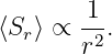
Solution 15: spherical spreading and conservation of radiated powerIn the far field,
Therefore the time-average Poynting flux satisfies
Doubling radius from 10λ to 20λ therefore gives
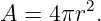
But a sphere has area
When radius doubles, area grows by a factor of four. Thus the quarter-sized local power density is spread across four times the area, leaving
unchanged. The 1∕r2 law is therefore precisely what conservation of radiated power requires for a freely expanding spherical wave.
Solution 16: Julia sweep of field zones and radiation patternOne implementation is supplied with the bundle as EM23E1_hertzian_sweep.jl. Its essential calculations are
using Printf

kr = 10 .^ range(log10(0.05), log10(30.0), length=300)
induction_ratio = 1.0 ./ kr
reactive_ratio  = 1.0 ./ kr.^2

theta = range(0.0, pi, length=2001)
pattern = sin.(theta).^2

# trapezoidal integral of sin^3(theta)
y = sin.(theta).^3
integral = sum((y[1:end-1] .+ y[2:end]) .* diff(theta) ./ 2)

ell_over_lambda = 10 .^ range(-3.0, -1.0, length=200)
Rrad = 80*pi^2 .* ell_over_lambda.^2

@printf("integral sin^3(theta) dtheta = %.8f\n", integral)
@printf("expected                         = %.8f\n", 4/3)
@printf("Rrad at ell/lambda=1/50         = %.6f ohm\n",
        80*pi^2*(1/50)^2)
The main checks are
and
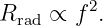
The numerical sweep should also show the slopes implied by 1∕(kr), 1∕(kr)2, and the quadratic scaling Rrad ∝ (ℓ∕λ)2.
What EM23E1 adds to the seriesEM23 established the radiation formulas. EM23E1 makes them operational. The central calculation chain is
The exercises also make the field-zone hierarchy quantitative through the single dimensionless distance kr. The next antenna article can now treat radiation intensity as the starting point for antenna directivity, efficiency, gain, EIRP, and receive effective aperture.
References
References
[1] Constantine A. Balanis, Antenna Theory: Analysis and Design, 4th ed., Wiley, 2016. [2] Warren L. Stutzman and Gary A. Thiele, Antenna Theory and Design, 3rd ed., Wiley, 2012. [3] David J. Griffiths, Introduction to Electrodynamics, 4th ed., Cambridge University Press, 2017. [4] John D. Jackson, Classical Electrodynamics, 3rd ed., Wiley, 1999. "example of Electromagnetic Waves, Antennas, and RF: Radiation from Time-Varying Currents and the Hertzian Dipole" is owned by bloftin.
This object's parent. Cross-references: effective aperture, antenna directivity, square, Conductor, representations, Wavenumber, program, boundary, solid, relation, induction, magnitudes, phase factor, resistance, Power, flux, radiation, formulas, EM23 This is version 1 of example of Electromagnetic Waves, Antennas, and RF: Radiation from Time-Varying Currents and the Hertzian Dipole, born on 2026-10-10. Object id is 1450, canonical name is ExampleOfElectromagneticWavesAntennasAndRFRadiationFromTimeVaryingCurrentsAndTheHertzianDipole. Accessed 12 times total. Classification:
|
|
|
|
Pending Errata and AddendaNone.
|
DiscussionNo messages.
|
Interact |
![[parent]](https://images.physicslibrary.org/images/uparrow.png)


























































![[ u3 ]
u − ---
3](https://images.physicslibrary.org/cache/objects/1450/make4ht/ExampleOfElectromagneticWavesAntennasAndRFRadiationFromTimeVaryingCurrentsAndTheHertzianDipole86x.png)