Electromagnetic Waves, Antennas, and RF: Faraday’s Law and Electromagnetic Induction -
Exercises and Complete Worked Solutions
This companion article extends EM13 with a second self-study problem set on magnetic flux,
Faraday’s law, Lenz’s law, motional emf, induced Electric Fields, and the Maxwell–Faraday
equation. All exercises are stated first. Complete worked solutions follow in Part II.
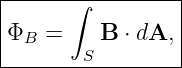
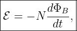
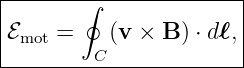
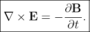
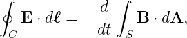
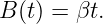
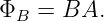
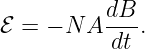
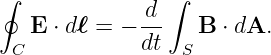
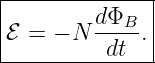
The principal relations are
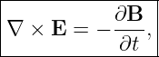
and, for a fixed contour and surface,
For a uniform field through a flat loop,
where 𝜃 is measured from the chosen surface normal. These conventions follow EM13 and standard
treatments of electromagnetic induction [1, 2, 3, 5].
How to use this problem set
Attempt every exercise in Part I before reading Part II. For each induction problem:
- choose and state the surface-normal orientation;
- determine the signed magnetic flux;
- differentiate the flux before applying the minus sign;
- use Lenz’s law or the Lorentz force to interpret direction;
- distinguish transformer emf from motional emf when the circuit itself moves.
Part I: Exercises
Exercise 1: signed magnetic flux and reversed orientation
A flat loop has area
A uniform magnetic field has magnitude
and the angle between B and the chosen surface normal is
Find:
- the signed magnetic flux;
- the signed flux after reversing the surface-normal convention.
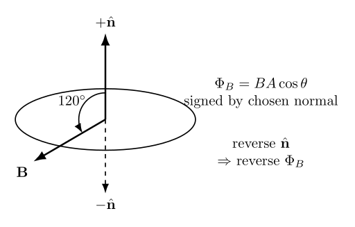
Figure. The sign of magnetic flux depends on the chosen surface normal. Reversing the
orientation reverses the sign of ΦB without changing the physical field.
Exercise 2: induced emf in a multiturn coil
A 120-turn coil has area per turn
The magnetic field is perpendicular to the coil and points along the chosen positive normal. It
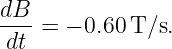
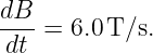
decreases at the constant rate
Find the signed emf for the positive loop traversal associated with the chosen normal.
Exercise 3: Lenz-law direction
A circular conducting loop is viewed from the front. An external magnetic field points into the
page and is increasing.
Determine:
- the direction of the induced magnetic field;
- whether the induced current is clockwise or counterclockwise.
Exercise 4: rotating-coil generator
A 60-turn coil of area
rotates at frequency
in a uniform field
Take the magnetic flux to be maximum and positive at t = 0.
Find:
- the angular frequency ω;
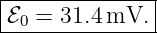
- the peak emf ℰ0;
- the instantaneous emf at t = 1∕(8f).
Exercise 5: motional emf and rod polarity
A conducting rod of length
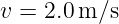
is oriented along the y axis and moves with
through
Find:
- the motional-emf magnitude;
- the direction of the magnetic force on positive charge;
- which end of the rod becomes positive.
Exercise 6: energy balance in a sliding-rod circuit
A rod of length
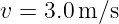
slides at constant speed
through a uniform magnetic field
The rod completes a circuit with total resistance
Assume the rod, velocity, and field are mutually perpendicular.
Find:
- the motional emf;
- the current magnitude;
- the electrical power dissipated;
- the magnetic drag-force magnitude on the rod;
- the mechanical power required to maintain constant speed.
Exercise 7: loop entering a magnetic-field region
A rectangular loop of height
and width
moves to the right at constant speed
into a region containing a uniform magnetic field
directed into the page. At t = 0, the leading edge of the loop just enters the field region.
Find:
- the overlap area A(t) while 0 < t < w∕v;
- the magnetic-flux magnitude during entry;
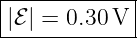
- the emf magnitude during entry;
- the emf after the loop is completely inside a uniform field region.
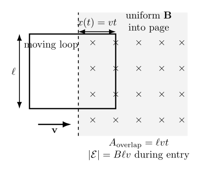
Figure. As the loop enters the magnetic-field region, its overlap area changes even though
the field itself is static.
Exercise 8: changing loop area in a static field
A loop remains perpendicular to a uniform static magnetic field
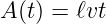
Its area changes according to
in square metres, with t in seconds.
Find the emf magnitude and identify the physical origin of the flux change.
Exercise 9: induced electric field inside a changing-field region
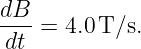
A spatially uniform magnetic field fills a circular region and changes at the constant
rate
Find the induced electric-field magnitude on a circular contour of radius
that lies entirely inside the changing-field region.
Exercise 10: induced electric field outside a changing-field region
A changing magnetic field occupies a circular region of radius
and changes at the rate
Find the induced electric-field magnitude on a circular contour of radius
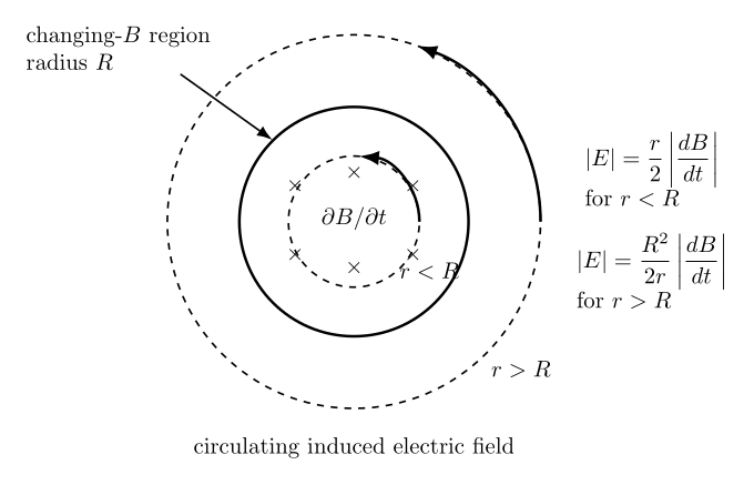
Figure. A changing magnetic field produces a circulating electric field. The enclosed
magnetic-flux area differs for observation contours inside and outside the changing-field
region.
Exercise 11: derive the Maxwell–Faraday differential equation
Starting from the stationary-contour integral law
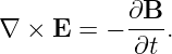
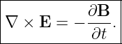
use Stokes’ theorem to derive
State the assumption that permits the time derivative to be moved inside the surface
integral.
Exercise 12: local curl from a specified time-varying field
At a particular spatial region, the magnetic field is
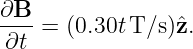
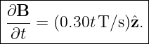
with t in seconds.
Find:
- ∂B∕∂t;
- ∇× E at t = 2.0 s;
- the local circulation sense viewed from the +z side.
Exercise 13: simultaneous field change and geometry change
A rectangular loop enters a magnetic-field region. During the interval of interest, the overlap area
is
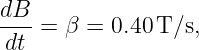
and the field magnitude is also increasing according to
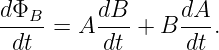
Use
Find at
the magnitudes of:
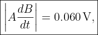
- the contribution AdB∕dt;
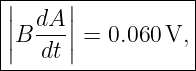
- the contribution B dA∕dt;
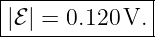
- the total emf.
Exercise 14: RF loop receiving-field preview
A 10-turn loop has area per turn
A locally uniform sinusoidal magnetic field has magnitude
where
The field makes an angle
with the loop normal.
Ignoring loading, self-inductance, radiation, and spatial variation over the loop, find:
- the flux per turn;
- an expression for the induced emf;
- the peak emf magnitude.
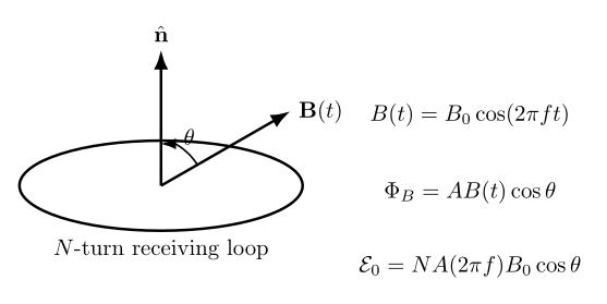
Figure. A simple receiving-loop preview. Only the magnetic-field component normal to
the loop contributes to the linked magnetic flux in this lumped approximation.
Part II: Complete Worked Solutions
Solution 1: signed magnetic flux and reversed orientation
For a uniform field through a flat loop,
Therefore,
| ΦB | = (0.40)(1.5 × 10⁻²) cos 120∘ | (44)
|
| = (0.40)(1.5 × 10⁻²)(−0.5) | (45)
|
| = −3.0 × 10⁻³ Wb. | (46) |
Thus,
Reversing the surface normal changes the angle from 120∘ to 60∘, so the sign reverses:
The physical field and loop are unchanged. Only the orientation convention changes.
Solution 2: induced emf in a multiturn coil
Because the field is normal to the coil and points along the chosen positive normal,
For N turns,
Therefore,
| ℰ | = −(120)(2.5 × 10⁻³)(−0.60) | (51)
|
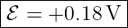
| = +0.18 V. | (52) |
Hence,
for the positive loop traversal associated with the chosen normal.
Solution 3: Lenz-law direction
The external magnetic field points into the page and is increasing. The induced response must
oppose that increase, so the induced field points out of the page.
Therefore,
A counterclockwise current produces a magnetic field out of the page by the right-hand rule.
Thus,
Solution 4: rotating-coil generator
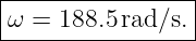
The angular frequency is
Therefore,
| ω | = 2π(30) | (57)
|
| = 188.5 rad/s. | (58) |
So,
With maximum positive flux at t = 0,
so
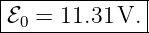
The peak emf is
| ℰ0 | = (60)(4.0 × 10⁻³)(0.25)(188.5) | (62)
|
| = 11.31 V. | (63) |
Thus,
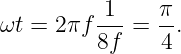
At
the phase is
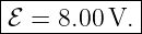
Therefore,
| ℰ | = 11.31 sin  | (67)
|
| = 8.00 V. | (68) |
Hence,
Solution 5: motional emf and rod polarity
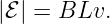
For mutually perpendicular rod, velocity, and field,
Thus,
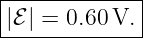
| |ℰ| | = (0.30)(0.50)(4.0) | (71)
|
| = 0.60 V. | (72) |
Therefore,
For positive charge,
| v × B | ∝x ×z | (74)
|
| = −y. | (75) |
So positive charge is driven toward the −y end of the rod:
Therefore, the −y end becomes positive relative to the +y end.
Solution 6: energy balance in a sliding-rod circuit
The motional emf is
| ℰ | = BLv | (77)
|
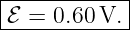
| = (0.50)(0.40)(3.0) | (78)
|
| = 0.60 V. | (79) |
Thus,
The current magnitude is
| I | =  | (81)
|
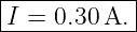
| =  | (82)
|
| = 0.30 A. | (83) |
Hence,
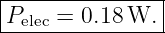
The electrical power dissipated is
| Pelec | = I2R | (85)
|
| = (0.30)2(2.0) | (86)
|
| = 0.18 W. | (87) |
So,
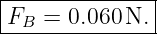
The magnetic force magnitude on the current-carrying rod is
| FB | = ILB | (89)
|
| = (0.30)(0.40)(0.50) | (90)
|
| = 0.060 N. | (91) |
Therefore,
The external force required to maintain constant speed has equal magnitude and opposite
direction. Its mechanical power is
| Pmech | = Fv | (93)
|
| = (0.060)(3.0) | (94)
|
| = 0.18 W. | (95) |
Thus,
This equality demonstrates the energy-conservation content of Lenz’s law for the idealized
circuit.
Solution 7: loop entering a magnetic-field region
During entry, the overlap width is
Therefore the overlap area is
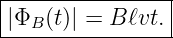
The flux magnitude is
Thus,
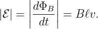
The emf magnitude is
Numerically,
| |ℰ| | = (0.60)(0.25)(2.0) | (102)
|
| = 0.30 V. | (103) |
Therefore,
while the loop is entering.
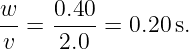
The entry interval lasts
After the loop is fully inside a spatially uniform static field, the flux is constant, so
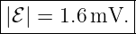
Solution 8: changing loop area in a static field
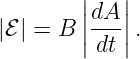
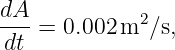
The field is static, but the area changes:
Therefore,
Since
we obtain
| |ℰ| | = (0.80)(0.002) | (110)
|
| = 1.6 × 10⁻³ V. | (111) |
Thus,
The flux change is caused by changing circuit geometry rather than by a time-varying magnetic
field.
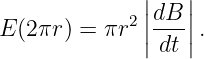
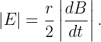
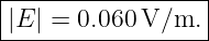
Solution 9: induced electric field inside a changing-field region
For a circular contour of radius r entirely inside the changing-field region,
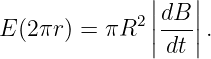
Therefore,
Substitute:
| |E| | = 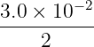 (4.0) (4.0) | (115)
|
| = 6.0 × 10⁻² V/m. | (116) |
Hence,
Solution 10: induced electric field outside a changing-field region
For r > R, only the magnetic-field region contributes to the flux:
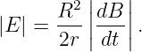
Therefore,
Substitute:
| |E| | = 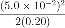 (6.0) (6.0) | (120)
|
| = 3.75 × 10⁻² V/m. | (121) |
Thus,
Solution 11: derive the Maxwell–Faraday differential equation
Start from
By Stokes’ theorem,
For a fixed surface, the time derivative may be moved inside the integral:
Therefore,
Because the surface is arbitrary,
The required assumption is that the chosen contour and spanning surface are fixed in space while
taking the time derivative.
Solution 12: local curl from a specified time-varying field
The field is
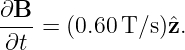
Differentiate:
Thus,
At t = 2.0 s,
Therefore,
A curl in the −z direction corresponds to clockwise local circulation when viewed from the +z
side.
Solution 13: simultaneous field change and geometry change
The magnetic flux magnitude is
Therefore,
At t = 0.50 s,
and
Also,
and
The field-change contribution is
A | = (0.15)(0.40) | (139)
|
| = 0.060 V. | (140) |
The geometry-change contribution is
B | = (0.20)(0.30) | (141)
|
| = 0.060 V. | (142) |
Therefore,
and the total emf magnitude is
Solution 14: RF loop receiving-field preview
The magnetic-field component normal to the loop is
The flux per turn is therefore
For N turns,
| ℰ(t) | = −N | (148)
|
| = NAB0(2πf) cos 𝜃 sin(2πft). | (149) |
Thus,
The peak magnitude is
Substitute
Then
| ℰ0 | = (10)(1.0 × 10⁻⁴)(1.0 × 10⁻⁶)(2π)(1.0 × 10⁷)(0.5) | (153)
|
| = 3.14 × 10⁻² V. | (154) |
Hence,
This is a lumped induction preview only. A practical RF loop antenna additionally requires
impedance, Resonance, loading, radiation, polarization, and full-wave analysis.
Common mistakes
- Using the angle from the plane rather than the surface normal in BA cos 𝜃.
- Ignoring the sign change when the surface orientation is reversed.
- Using Lenz’s law as “opposes the field” instead of “opposes the change in flux.”
- Applying BLv without checking the cross-product geometry.
- Forgetting that a static magnetic field can still produce emf if the circuit geometry
changes.
- Treating transformer emf and motional emf as the same local mechanism.
- Using the full observation-contour area for the outside induced-E problem when the
magnetic field occupies only radius R.
- Forgetting the factor N for a multiturn coil.
Reinforcement summary
Faraday’s law is fundamentally a flux-change law:
Flux can change because the field changes, the circuit geometry changes, the orientation changes,
or several of these occur simultaneously. The local field form,
shows that a time-varying magnetic field produces circulating electric-field structure even when no
wire is present.
These results form one half of the dynamical curl coupling required for electromagnetic waves. The
complementary time-dependent magnetic-curl equation will arise from Maxwell’s correction to
Ampère’s law.
References
[1] David J. Griffiths, Introduction to Electrodynamics, 4th ed., Cambridge University
Press, 2017.
[2] Edward M. Purcell and David J. Morin, Electricity and Magnetism, 3rd ed.,
Cambridge University Press, 2013.
[3] Samuel J. Ling, Jeff Sanny, and William Moebs, University Physics, Volume 2,
OpenStax, 2016, sections on electromagnetic induction, Faraday’s law, motional emf, and
generators.
[4] Richard P. Feynman, Robert B. Leighton, and Matthew Sands, The Feynman Lectures
on Physics, Volume II, Addison-Wesley, 1964, chapters on electromagnetic induction and
Maxwell’s equations.
[5] Massachusetts Institute of Technology, 8.02 Physics II: Electricity and Magnetism,
MIT OpenCourseWare, materials on Faraday’s law, Lenz’s law, motional emf, and
electromagnetic induction.

![[parent]](https://images.physicslibrary.org/images/uparrow.png)