0.1 Classical differential geometry
Differential geometry studies geometrical objects using techniques of calculus. In fact, its early
history is indistiguishable from that of calculus — it is a matter of personal taste whether
one chooses to regard Fermat’s method of drawing tangents and finding extrema as a
contribution to calculus or differential geometry; the pioneering work of Barrow and
Newton on calculus was presented in a geometrical language; Halley’s 1696 paper in
which he announces his discovery that ∫
 = log x + C is entitled quadrature of the
hyperbola.
= log x + C is entitled quadrature of the
hyperbola.
It is only later on, when calculus became more algebraic in outlook that one can begin to make a
meaningful separation between the subjects of calculus and differential geometry. Early differential
geometers studied such properties of curves and surfaces such as: computing their lengths and
areas, finding tangents, constructing evolute, involute, and pedal curves, studying curvature and
osculating circles, and finding envelopes and orthogonal curves to a given family of curves. Of the
various objects they studied, the cycloid deserves special mention. Originally discovered by Galileo,
it seems to have been studied by just about every seventeenth century mathematician, much more
than any other curve. Also, it is worth mentioning that the deep connections between
differential geometry and mechanics which play a prominent role in contemporary theoretical
physics also have their origin at this time — for instance, the fact that the problem of
geodesics on surfaces is related to the acceleration of particles was already to known to the
Bernoullis, even though the significance of this similarity was not fully appreciated until
Einstein.
0.2 Intrinsic geometry
A major turning point in differential geometry is marked by the appearance of Gauss’ memoir
“Disquisitiones generales circa superficies curvas”. In this memoir, Gauss first proposes the
intrinsic point of view in geometry. Since his idea of has intrinsic geometry has completely changed
the outlook of geometry, it might not be inappropriate to spend some time discussing
it.
Ordinarily, when we think of a surface such as a cylinder or a sphere, we concieve of a locus in
space (ℝ3). However, imagine that, like blind ants crawling on a sheet, we were confined to a
surface and had no direct knowledge of the space in which the surface was situated. What could we
conclude about the surface on which we live? Obviously, such constructions as Normals to the
surface or osculating spheres which are situated in the ambient space would be meaningless to us.
However, we would be still able to speak of the lengths of curves drawn on the surface, the
angle between curves, and areas of portions of our surface since these can be defined in
terms of measurements which are made on the surface without recourse to the ambient
space.
Considering differential geometry from this point of view, one comes to several interesting
conclusions. One is that certain surfaces, such as a portion of a plane and a portion of a cylinder
are indistinguishable from the intrinsic point of view. This result can be something of a surprise
because one is usually accostomed to thinking of planes and cylinders as rather different sorts of
objects — planes are flat while cylinders are curved.
By itself this discovery is interesting, but perhaps not enough to fire a revolution in geometry.
Hearing of it, one might come to the conclusion that intrinsic measurements alone are not sufficient
to describe the geometry of a surface and, hence, the subject of intrinsic geometry is uninteresting.
Further study shows that this is not the case. While one may not be able to distinguish a plane
from a cylinder on the basis of intrinsic measurements alone, it is possible to distinguish a portion
of plane from a portion of sphere solely on the basis of intrinsic measurements. Even more,
it is possible to distinguish portions of spheres of different radii intrinsically. This, of
course, is of interest not only because it shows that the study of intrinsic geometry is
non-trivial, but because a quantity such as the radius of a sphere which is defined as the
distance from a point on the sphere to a point not on the surface (namely, the centre of
the sphere) can, in fact, be deduced solely from measurements on the surface of the
sphere.
To prove such results, Gauss used the concept of curvature. Since the idea of curvature, in one
from or another, plays an important role in differential geometry to this day, let us say a few words
about this key concept. The concept of curvature was developed in the eighteenth century as a
measure how much a given curve or a surface deviates from being a straight line or a plane. In the
case of a curve, the curvature may be defined as the second derivative of the normal
angle with respect to arclength. In the case of a surface, the situation is a little more
complicated — to describe the direction of the normal vector, one needs two angles instead of
one and one can choose to compute their directional derivatives along any direction
tangent to the surface. Because of this, one obtains a 2 × 2 matrix of partial derivatives
instead of a single number. If one changes the coordinates used to describe the ambient
space, then the components of this matrix will undergo a linear transformation. To
obtain a quantity which does not depend on an arbitrary choice of coordinates and hence
can be seen as describing geometric properties of the surface, one should consider the
eigenvalues of this matrix. These eigenvalues are known as the principal curvatures of the
surface.
The remarkable theorem which Gauss proved was that, whilst the principal curvatures cannot be
determined from intrinsic measurements alone, their product can. This result, for instance, can be
used to explain the facts we mentioned about planes, cylinders, and spheres. For a plane, the two
principal curvatures equal zero. For a cylinder, one principal curvature is zero and the other is
positive. For a sphere, both principal curvatures are equal and positive. Since the product equals
zero for both the plane and the cylinder it is plausible that they are indistinguishable
intrinsically. Since it is not zero for the sphere, it follows from Gauss’ theorem that the
intrinsic geometry of the sphere could not possibly be the same as that of the plane and
cylinder.
0.3 The concept of a manifold
The discovery of intrinsic geometry led thoughtful geometers such as Riemann (who was a student
of Gauss), Clifford, and Mach to the conclusion that a “right and natural” approach
to geometry should regard surfaces as geometrical spaces in their own right on a par
with Euclidean and projective space. In the terminology of the mediaeval scholastic
philosophers, one may say that they regarded the intrinsic properties of surfaces as “essential”
and extrinsic properties as “accidental”. To properly develop geometry from such a
viewpoint, they needed to start with a definition of surface which made no reference to
any sort of ambient space. Their quest for such a definition led to the concept of a
manifold.
The genesis of this concept can be seen as a diasappearing act akin to that of the Chesire cat —
just as the grin is all that remains of the cat when the cat disappears, so too a manifold is what
remains when one starts with a parameterized surface and the space in which the surface is
situated disappears.
A parameterized surface may be decribed as a suitable subset S ∈ ℝ3 together with a smooth
bijective map from an open subset of ℝ2 to S (which is called a parameterization of the surface).
Moreover, (pay careful attention because this will turn out to be the key fact that makes the
concept of a manifold possible) one can describe the same surface using many different
parameterizations. Given two parameterizations ϕ: D1 ⊂ ℝ2 → S and ψ: D
2 ⊂ ℝ2 → S of the
same portion of surface, the two will be related by reparametrization; that is to say there exists a
smooth bijection gϕψ: D2 → D1 such that ψ = ϕ ∘ gϕψ.
By contrast, a manifold may be understood as a “parameterized set”. That is to say, a
n-dimensional manifold M is a set together with a set of bijective maps from open sets of ℝn to M
(which are called coordiante maps). As in the case of parameterized surfaces, a coordinate map
need not have the whole of M as its range. Moreover, we require that if two coordinate maps
ϕ: D1 ⊂ ℝ2 → M and ψ: D
2 ⊂ ℝ2 → M describe the same subset of the manifold, then there
exists a smooth bijective map gϕψ: D2 → D1 such that ψ = ϕ ∘ gϕψ. (Such a map is known as a
coordinate transformation map or a transition function.) To make this definition completely
correct, we require a few more technical assumptions but, in keeping with the spirit of this
expsition, we shall not discuss them here and instead refer the reader to the entry notes on the
classical definition of a manifold for a careful definition which takes technicalities into
account.
As is obvious from the definition, if we make the further assumption that the objects of our set be
points of Euclidean space and that the correspondence between points and pairs of numbers
be continuous, we recover the definition of parameterized surface. However, we choose
to refrain from making any asumption about the nature of the elements of our set.
This freedom is exactly what allows us to regard two surfaces with the same intrinsic
geometry as the same manifold — to obtain one surface, we specify one mapping of our set
into Euclidean space one way and to obtain the other surface we specify a different
mapping.
Objects other than surfaces can be manifolds. Most obviously, the Euclidean plane itself is a
manifold since its points can be described by pairs of real numbers according to various coordiante
systems (Cartesian coordinates, polar coordinates, etc.) Thus, the concept of manifold fulfills the
desire of its inventors that Euclidean space and surfaces be of the same ontological
status.
Less obviously and more curiously, the set of functions which satisfy the differential
equation
is also a two-dimensional manifold! The reason is that we can specify a solution of this equation
uniquely by giving the values of f and f′ at a particular value of t and, by the theorem on
continuous dependence on initial conditions, f(t1) and f′(t1) can be expressed as a continuous
functions of f(t2) and f′(t2) for any two numbers t1,t2 ∈ ℝ.
Another example of a manifold is the group of affine transforms of the line. Recall (or look back at
the section on affine geometry above!) that an affine transformation is of the form x ax + b.
Hence, such a transform is specified by giving the two real numbers a and b. A group like this one
which also happens to be a manifold is called a Lie group. The study of Lie groups
forms an important branch of group theory and is of relevance to other branches of
mathematics.
ax + b.
Hence, such a transform is specified by giving the two real numbers a and b. A group like this one
which also happens to be a manifold is called a Lie group. The study of Lie groups
forms an important branch of group theory and is of relevance to other branches of
mathematics.
Because of examples like the two just exhibited, it has been possible to apply the techniques of
differential geometry in some rather unlikely settings. Once geometric notions like tangent spaces
and curvature have been defined for manifolds (we shall indicate how this is done in the next
section) then one can speak of such things as the tangent space to the set of solutions of a
differential equation or the curvature of a group. While this may sound like a parlor stunt to
demonstrate the generality of our definitions, it is more than that. By applying the techniques of
differential geometry in such unlikely settings, mathematicians have been able to win insights and
prove results about differential equations, groups and other mathematical objects which otherwise
seemed intractable.
Before moving on to the next section, it might be worth pointing out that, when speaking of
manifolds, it is customary to refer to the elements of the set as points and the real numbers which
label them as points. The reader should keep in mind that this is merely customary terminology
which derives from thinking of manifolds as a generalization of parameterized surfaces and should
no way be understood as suggesting that the elements of the set which comprise our manifold
resemble points of a surface. As the examples show, they may be functions, transformations, or
other mathematical objects.
0.4 Structures on manifolds
In order to discuss such geometric notions as angles and lengths and perform interesting geometric
constructions, one needs to equip one’s manifold with suitable structures. In classical differential
geometry, these structures were provided by the ambient space, but now that the ambient space
has disappeared, they must put in by hand.
In placing structures on a manifold, the notion of reparameterization or change of coordinates
which was built into the definition of manifold plays a crucial role. To explain how the process of
imposing structures proceeds, let us start with a simple example — tangent vectors on a manifold.
In classical differential geometry, a tangent vector v to a surface S at a point p ∈ S is simply a
vector in Euclidean space whose direction happens to be tangent to the surface at the point p. We
could represent it graphically an arrow with its tail at p which points along a tangent to the
surface.
Of course, this description won’t do if we don’t have an ambient space in which to draw our arrow.
Therefore, we need to look for a different description of our tangent vector. One possibility is to
consider a description of the vector in terms of its components. However, to define the components
of a vector, one needs a basis. If our surface is specified parametrically, there is a natural choice of
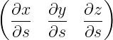
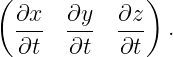
basis vectors, namely
and
Of course, if we choose a different parameterization, we obtain a different pair of basis vectors.
However, we can express one pair in terms of the other pair using the chain rule. Thus, if a
tangent vector v has components  with respect to the basis corresponding to the
parameterization in terms of parameters s and t, it will have components
with respect to the basis corresponding to the
parameterization in terms of parameters s and t, it will have components  with respect
to the basis corresponding to the parameterization in terms of parameters s′ and t′,
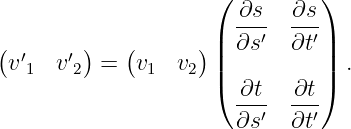
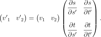
where
with respect
to the basis corresponding to the parameterization in terms of parameters s′ and t′,
where
These observations form the foundation of the definition of a tangent vector to a manifold. To
define a tangent vector v to a two-dimensional manifold M at a point p, we shall associate a pair of
numbers  to every coordinate system which describes p. The only restriction we impose is
that, given two coordinate systems, the pairs of numbers to be associated to these systems be
related by the transform
to every coordinate system which describes p. The only restriction we impose is
that, given two coordinate systems, the pairs of numbers to be associated to these systems be
related by the transform
To define other structures on the manifold, we can follow a similar recipe:
- Identify what sort of mathematical object will represent the structure in a coordinate
system. In the case of a tangent vector, this was an n-tuplet of real numbers.
- Identify how the this object is to transform under changes of coordinate system.
- Define the structure as an assignment of mathematical objects of the type identified
in item (1) to coordinate systems in such a way that the objects assigned to two
coordinate systems are related by the transform identified in item (2).
Using this procedure, one can define all sorts of structures on manifolds, of which we shall consider
only two more examples here. One example is the vector field. A vector field may be defined as the
assignment of a vector to every point in the manifold. Given a coordinate system, we may specify
such an entity by assigning an n-tuple of numbers to every point. In other words, in
a coordinate system our vector field is represented by an n-tuple of functions. Upon
making a change of coordinates, these n-tuples change according to the law presented
earlier.
The second example is the metric field. Recall that in our discussion of intrinsic geometry, we
considered measuring lengths and angles along the surface. Now, in Euclidean geometry,
we may define the notions of length and angle in terms of an inner product. A metric
field may be described as the assignment of an inner product for tangent vectors to
every point of the manifold. Given a basis, an inner product can be described by a
symmetric, positive-definite matrix. Hence, to define the notion of metric field, we will
consider the assignment of a symmetric, positive definite matrix of functions to every
coordinate system in such a way that the matrices assigned to two coordinate systems
are related according to the transformation law for inner products under a change of
basis.
Once we choose a metric field on a two-dimensional manifold, it becomes possible to study its
intrinsic geometry as defined in the last section.
0.5 Sheaves and bundles
In order to understand the toatality of all possible tangents vectors, metrics, etc. one typically
collects them into larger structures called sheaves and bundles. To understand how such
constructions proceed, we will start by examining the fundamental example of the tangent
bundle.
Last section, we desribed how a tangent vector is described in an intrinsic manner. Suppose we
now want to consider the totality of all tangent vectors to a manifold. We could start
by picking a point of the manifold and considering all tangent vectors based at that
point. Since it is meaningful to make linear combinations of tangent vectors with the
same basepoint, the set of all tangent vectors with a common basepoint forms a vector
space called the tangent space to the manifold at that point. As we saw earlier, vector
spaces are manifolds because one can impose coordinates on a vector space by choosing a
basis.
So our problem of describing the toality of all tangent vectors reduces to the problem of describing
the totality of all tangent spaces. We claim that they form a manifold. Basically, the reason for this
is that, to specify a tangent vector, we could give the coordinates of its basepoint with respect to a
coordinate system on the manifold and specify which vector by its coordnates with
respect to a basis for the tangent space at that point. This manifold whose points are
tangent vectors to a certain manifold is known as the tangent bundle of the orginal
manifold.
0.6 Back to Erlangen
When written, this entry will show how differential geometry may be understood as the study of
invariants of structures on manifolds under the group of diffeomorphisms. In terms of
this definition, we shall introduce such geometries as Riemannian geometry, conformal
geometry, Kahler geometry, symplectic geoemtry, contact geometry, teleparallel geometry,
gauge geometry, etc. much as Euclidean, affine, and projective geometry were introduced
above.
0.7 Differential invariants and local differential geometry
When written, this section will give the reader the flavor of the nuts and bolts of constructing the
invariants which are supposed to describe geometrical objects according to the Klein’s principles.
We shall mention such topics as Christoffel’s theorem and the Bianchi identitites and give some
idea of the sort of topics which one considers in local differential geometry.
0.8 Global differential geometry
When written, this section will describe the Gauss-Bonnet theorem and some of its modern
descendants such as characteristic classes and index theorems.
0.9 The algebraic viewpoint
When written, this entry outline how one may take the algebra of functions of a manifold as a
starting point and see that differential geometric notions correspond to algebraic constructions. In
fact, one may reformulate differential geometry as the study of invariants of an algebra under the
action of a group of automorphisms. Using this even more general definition, one arrives at such
novel topics as the differential geometry of finite-dimensional algebras and non-commutative
geometry.