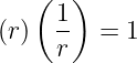
(work in progress)
1 BASIC TENSOR THEORY
Tensor analysis is the study of invariant objects, whose properties must be independent of the
coordinate systems used to describe the objects. A tensor is represented by a set of functions called
components. For an object to be a tensor it must be an invariant that transforms from one
acceptable coordinate system to another by the tensor rules.
Several examples of tensors are velocity vector, base vectors, metric coefficients for the length of a
line, Gaussian curvature, and the Newtonian gravitation potential.
Many of the important differential equations for physics, engineering, and applied mathematics can
also be written as tensors. Examples of differential equations that can be written in tensor
form are Lagrange’s equations of motion and Laplace’s equation. When an equation is
written in tensor form it is in a general form that applies to all admissible coordinate
systems.
1.1 Summation Notation
The summation notation used throughout this section will be of the type:
The superscripts on x are not powers; they are used to distinguish between the various x′s. In
rectangular Cartesian coordinates and vector notation, Equation 1 would be:
where,
x1 = x, x2 = y, x3 = z
a1 = i, a2 = j, a3 = k
With this interpretation of Equation 1.1 and the specific values for ai and xi as noted, sum S would
be:
For additional simplification, Einstein dropped the ∑
in Equation 1.1 and the summation is then
expressed
This short cut is referred to as Einstein notation or Einstein summation convention. Further, a
superscript index will indicate a contravariant tensor, while a subscript index will indicate a
covariant tensor.
The rank of a tensor is the sum of the covariant and contravariant indexes.
1.2 Relative Tensors
The term relative tensor is used to describe scalars that are transformed from one co-ordinate
system to another by means of the functional determinate known as the Jacobian. To illustrate this
concept, the differential increment of area(dA) is indicated in Fig. 1-1.
In cartesian coordinates (x, y) it is:
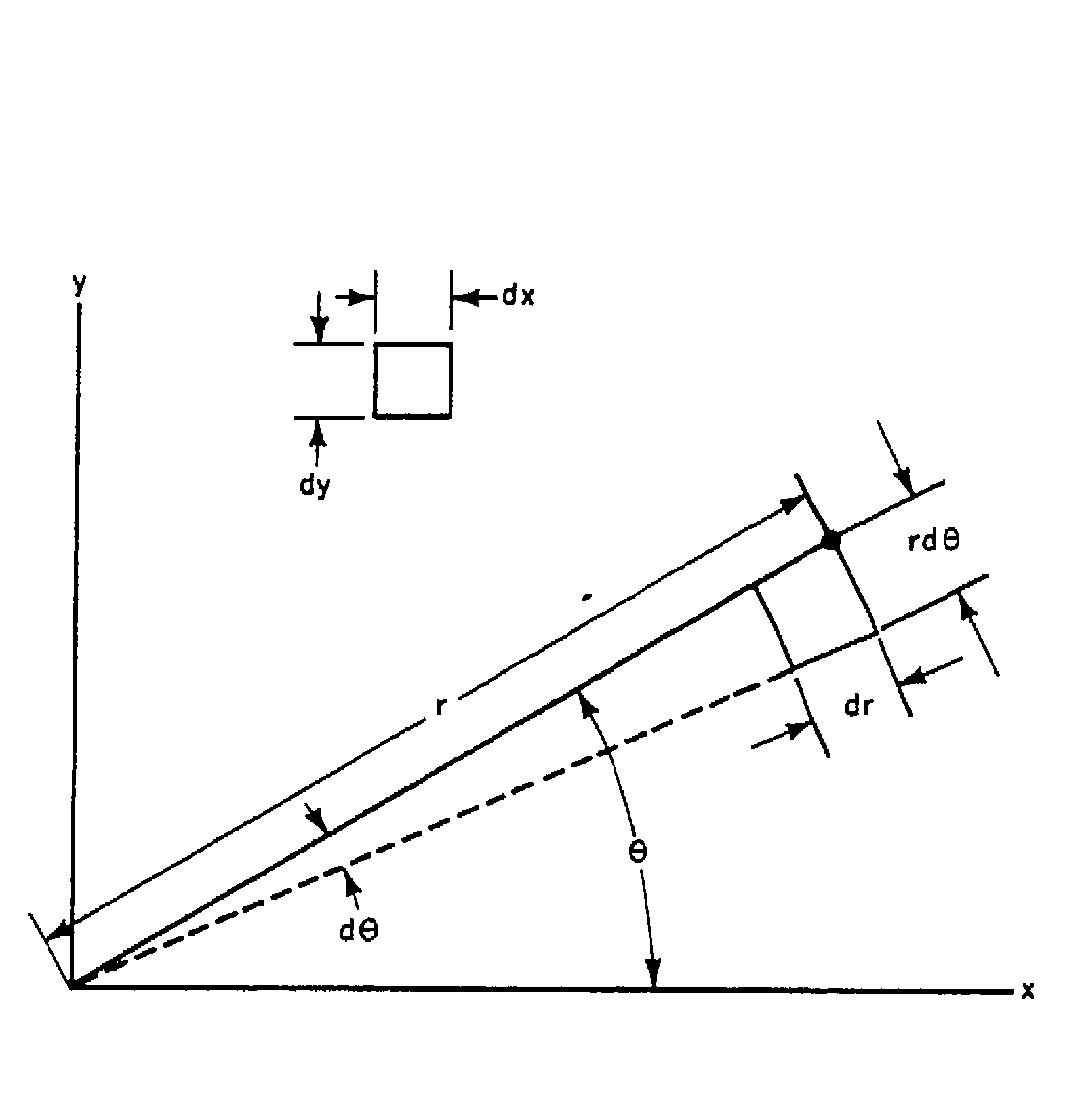
Fig. 1-1.
In polar coordinates (r, 𝜃) it is :
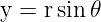
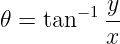
Now, the connection between the x, y cartesian coordinates and the r,𝜃 polar coordinates
is:
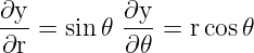
The Jacobian of the cartesian coordinates with respect to the polar coordinates is formed from the
following partial derivatives :
This set of partial derivatives are used to form the following Jacobian:
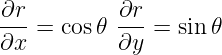
In the same manner, the Jacobian of polar cooordinates with respect to the cartesian coordinates is
formed from the following partial derivatives:
This set of partial derivatives are used to form the following Jacobian:
Now, returning to the expression for differential area in cartesian coordinates and polar
co-ordinates, the following equation can be written:
where,
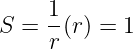
S = 1
S = r
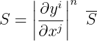
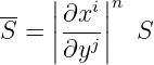
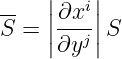
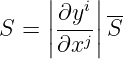
S and S are called relative tensors, as they are related by the equations:
Exponent n in Equations 4 and 5 is used to determine the Weight of a relative scalar. The
examples in this section are relative scalars having a weight equaling one; therefore, n = 1. An
absolute scalar has a weight of zero; i.e., n = 0. To illustrate Equation 4, we use the
values:
Equation 6 is the desired result.
Now the notion of relative tensors can be extended to volumes and mass. To illustrate this
concept, we start with the equation for an incremental mass in orthogonal cartesian
coordinates.
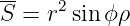
Now the incremental mass in spherical coordinates is written in terms of relative tensor
S:
S is evaluated by the relative tensor equation:
In this example S = ρ, where ρ is called the scalar density.
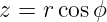
The geometrical relationship between the cartesian coordinates and the spherical co-ordinates is
indicated in Fig. 1-2. The corresponding mathematical relationship between the coordinates
is:
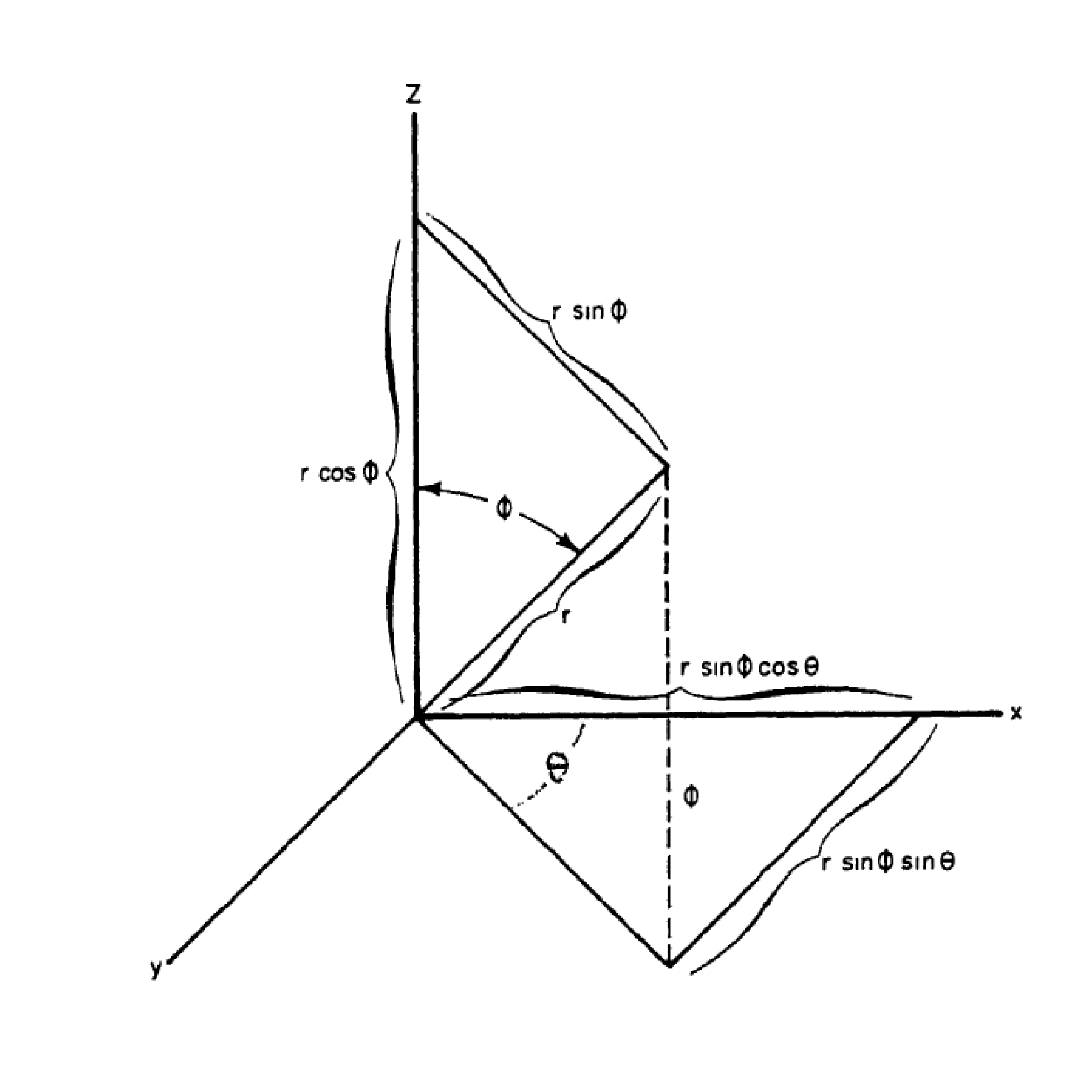
Fig. 1-2.
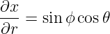
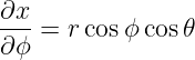
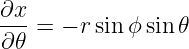
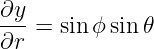
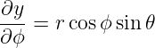
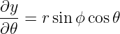
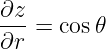
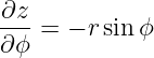
The partial derivatives for the Jacobian  are:
are:
Using these values, the resultant determinate is:
Now, Equation 5 can be evaluated:
and the equation for dM is:
Equation 11 is the desired result for dM. If the value for dM had been given initially in spherical
coordinates, the corresponding value in cartesian coordinates could be found by the
equation:
where,
1.3 Admissible Transformations
From the previous examples, it has been demonstrated that relative tensors transform from one
coordinate system to another by means of the functional determinate known as the
Jacobian. Since a relative tensor is defined to be a function of the Jacobian, a necessary and
sufficient condition for an admissible transformation of coordinates is that it is a member
of a set in which the Jacobian does not vanish. This condition is also necessary and
sufficient for absolute tensors. Therefore, the set of all admissible transformations of
co-ordinates form a group with non vanishing Jacobians. If notation  is used for
the Jacobian, the definition for an admissible transformation of co-ordinates can be
expressed:
is used for
the Jacobian, the definition for an admissible transformation of co-ordinates can be
expressed:
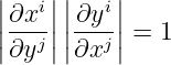
Another property of an admissible transformation is:
An example of Equation 15 can be found in Jacobian Equation 2 and 3.
1.4 N Dimensional Space
In general terms a coordinate system represents a one-to-one correspondence of a point or object
with a set of numbers. To measure distance, we can use a rectangular cartesian coordinate system.
This is called a metric manifold, or space of V 3.
Now, a space or manifold of N dimensions is expressed by the symbol V N; and it is a coordinate
system of N dimensions, if for each set of N numbers there is one corresponding point or
object.
A sub space V M where M = N − 1 is called a hypersurface. An example of a hypersurface in
Euclidean space is a plane. It is a hypersurface of V 2.
1.5 Contravariant Tensors
1.6 Covariant Tensors
1.7 Higher Rank and Mixed Tensors
1.8 Metric Tensors and the Line Element
1.9 Base Vectors
1.10 Associated Tensors and the Inner Product
1.11 Kronecker Deltas
This is a Derivative work from the public domain work of
”Principles and Applications of Tensor Analysis” By MATTHEW S. SMITH