ANY magnitude which has size, in the ordinary algebraic sense of the word, as well as direction in space, is termed a vector, whereas the common algebraic magnitudes, which have nothing to do with direction in space, which have no directional properties, but are each determined completely by a single (real) number, are called scalars. The typical case of a vector and, in fact, the intuitional representative of any vector, is a segment of a straight line of some definite length and of some definite direction in space, the size of the vector being represented by the length, and its direction by the direction of the straight line.

Thus, the displacement of a particle from some initial to some other final position is a vector, and is represented by the segment of the straight line joining the two positions and directed from the first to the second. Other examples of vectors are the instantaneous velocity of a particle, its acceleration, its momentum, the force acting on a particle, also the instantaneous rotational velocity of, say, a rigid body round a given axis, and so on. On the other hand, mass (in classical mechanics), temperature, vis viva, energy in general; gravitational, electric or magnetic potential (of fixed charges or magnets), mechanical or any other kind of work are all scalars.

The size of a vector, or magnitude (absolute value) apart from direction, is called its tensor, or sometimes intensity. Thus, the tensor of a vector is an essentially positive scalar.

Every vector can be determined completely by three scalar quantities, for instance, by its projections on any three fixed axes, orthogonal or oblique, but not coplanar, these projections being commonly called the vector’s components; for example, the components of a force or the components of a velocity. We also may use polar coordinates, that is to say, we may define the tensor of a vector by the scalar r, and the direction by two other scalars, i.e. by two angles 𝜃, ϕ, say the geographical latitude and longitude. In this way we get again three mutually independent scalars determining a single vector.

Obviously, such a decomposition of a vector into its three components or, more generally, into three mutually independent scalars, will in the majority of cases bring in some artificial elements, especially if the system of reference (axes, etc.) or the scaffolding constructed round the natural entities or phenomena be chosen quite at random without having anything in common with the essential characters of these entities or phenomena. Very often such a procedure gives rise to a hopeless complication of the resulting scalar formulae, a complication which does not arise from the intrinsic peculiarities of the phenomena in question, but is wholly artificial, a complication not due to Nature but to the (mathematizing) naturalist. Now, Nature is of herself wonderfully complicated; so that supplementary complication is not wanted.

This remark alone may suggest that to operate with vectors, each taken as a whole, without decomposing them into scalar components, may be more convenient and more simple, especially in those regions of research in which we are concerned mainly with vectors or directed magnitudes, as in Electromagnetism and in General Mechanics. But a true appreciation of the advantage of the vector method over the Cartesian (or scalar component) procedure is possible only when we see it actually at work, and the main object of each of the following chapters is to exhibit this working in Mechanics. Still more conspicuous is the service done by the vector method in Electromagnetism, especially in the hands of Oliver Heaviside, to whom also is due that simplified form of this mathematical method, which in its main features we shall now develop.

Definition I. By saying that two vectors are equal to one another we mean that their tensors are equal and that they have the same direction, or, what is the same thing, that their representative straight line-segments have the same lengths and are parallel to one another and similarly (not oppositely) directed; but the equality is independent of their position in space.

According to this definition, the shifting of a given vector parallel to itself is quite immaterial, or does not change the vector.

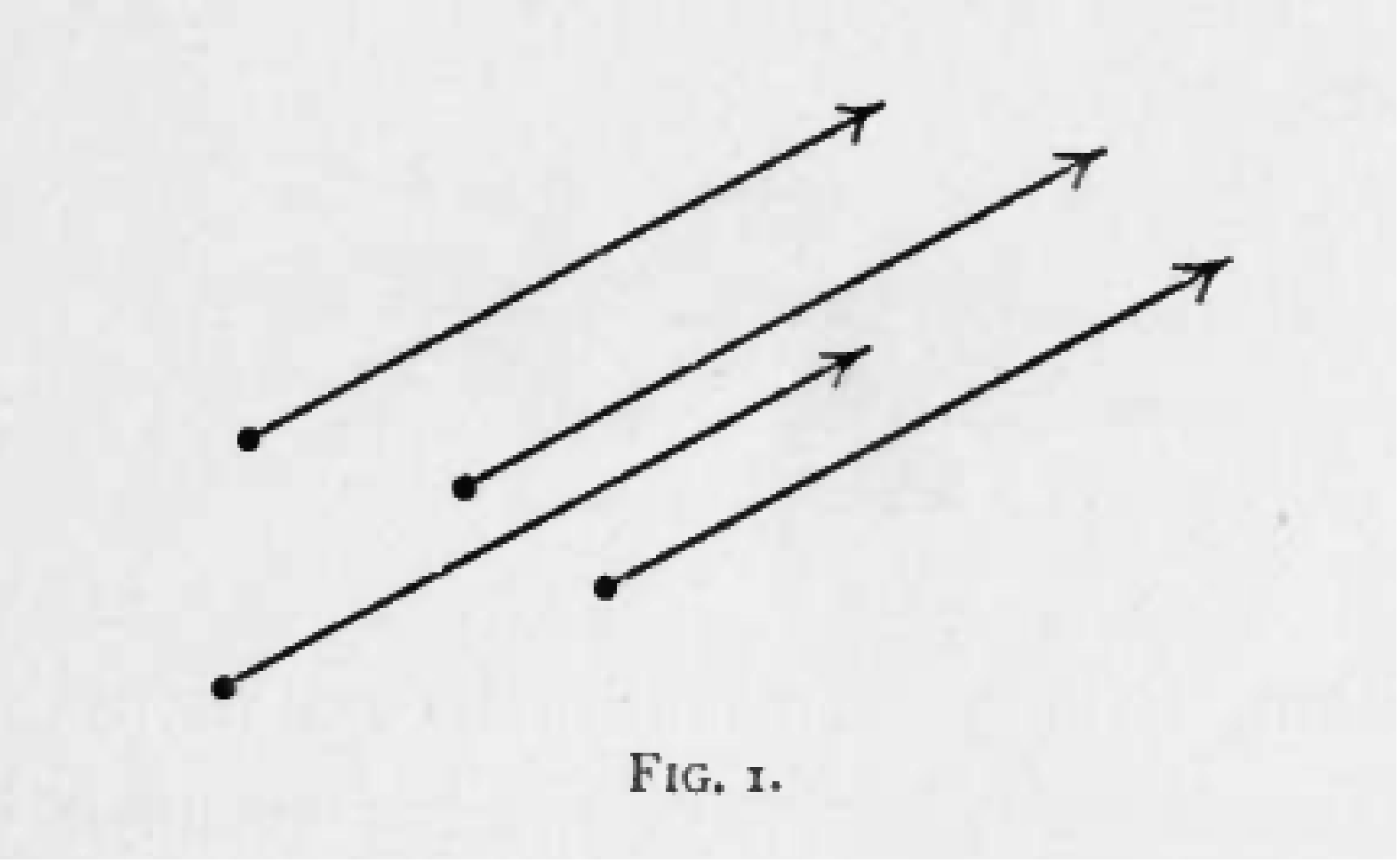
Thus, all the vectors represented on Fig. I. are to be considered as equal to one another. The parallel shifting of a vector, which by convention leaves it the same, is, of course, not confined to one plane.

Following the example of Heaviside and Gibbs vectors will be printed in bold, and their tensors will be denoted by the same letters printed in ordinary type (or simple italics). Thus

will be the tensors of the vectors

A, B, C

respectively.

If the tensor of a vector, say a, be equal to unity (in a given scale), i.e. if

then the vector a is called a unit-vector.

By the definition, every tensor is an absolute or positive number. It has, of course, the same denomination as the physical, or geometrical, quantity represented by the vector, i.e. if A be a velocity, then A signifies so many centimetres per second, and similarly in all other cases.

We pass now to the fundamental operations of vector algebra. These are : the addition of two vectors, and its inverse, the subtraction of one vector from another, and two different kinds of multiplication, the scalar and the vector multiplication of two vectors (scalar product and vector product). (The division, i.e. the quotient of two vectors, belongs to the Calculus of quaternions, due to Hamilton, and has nothing to do with Heaviside’s and Gibbs’ vector method to be developed here, notwithstanding that the latter has grown out of the former, historically.)

Let us begin with the operation of addition and its result, the sum of two vectors.

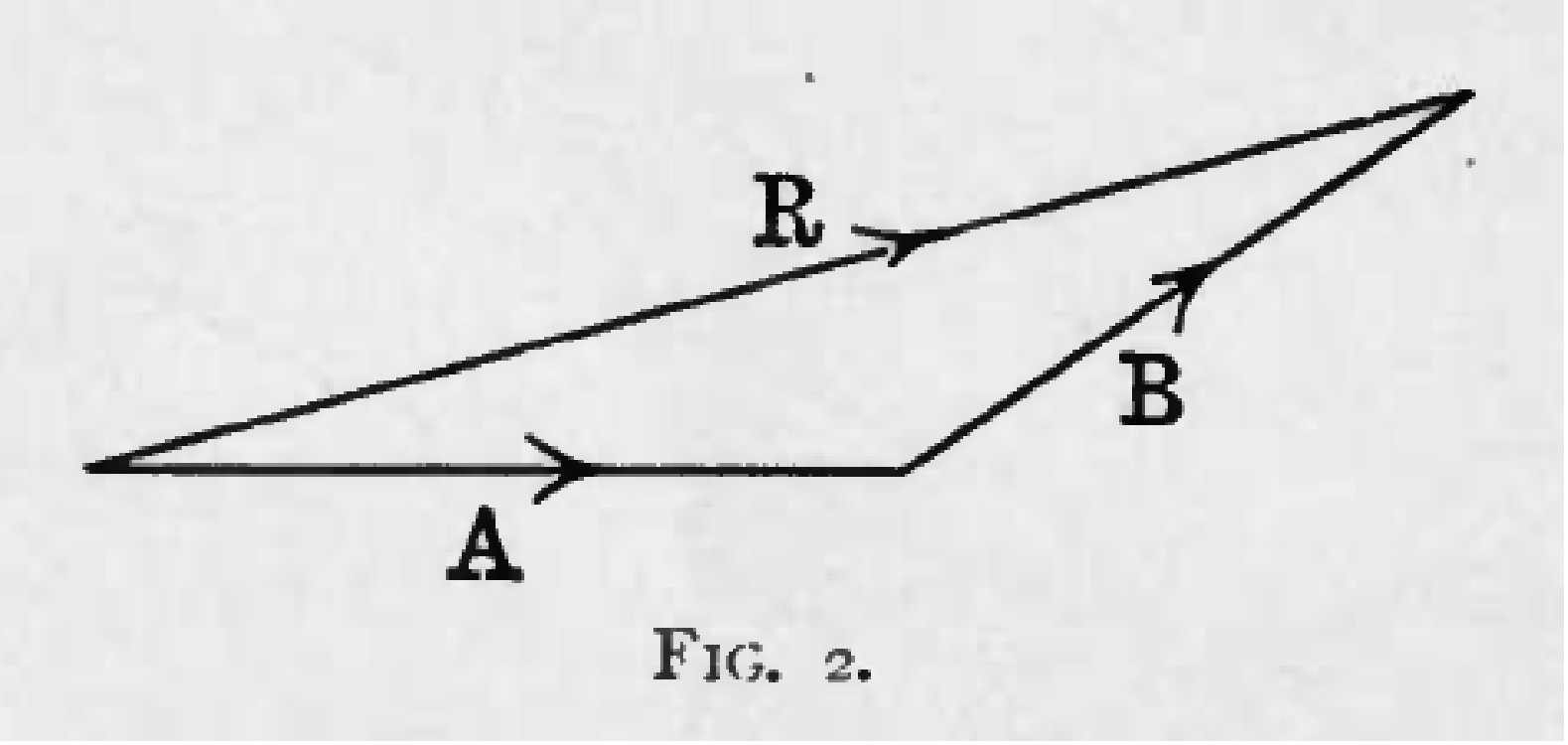
Definition II. If the end of the vector A coincides with the beginning of another vector B, then we call sum of A and B and denote by

a third vector R which runs from the beginning of A to the end of B (Fig. 2).

This definition of sum seems at first too narrow, as far as it appeals to the chain-arrangement of the two vectors; but in fact it embraces the concept of the sum of any two vectors. For, if B or its representative line be originally given in a quite arbitrary manner relatively to A, we can always shift it parallel to itself (which is allowed by Definition I.) till its beginning is brought into coincidence with the end of A.

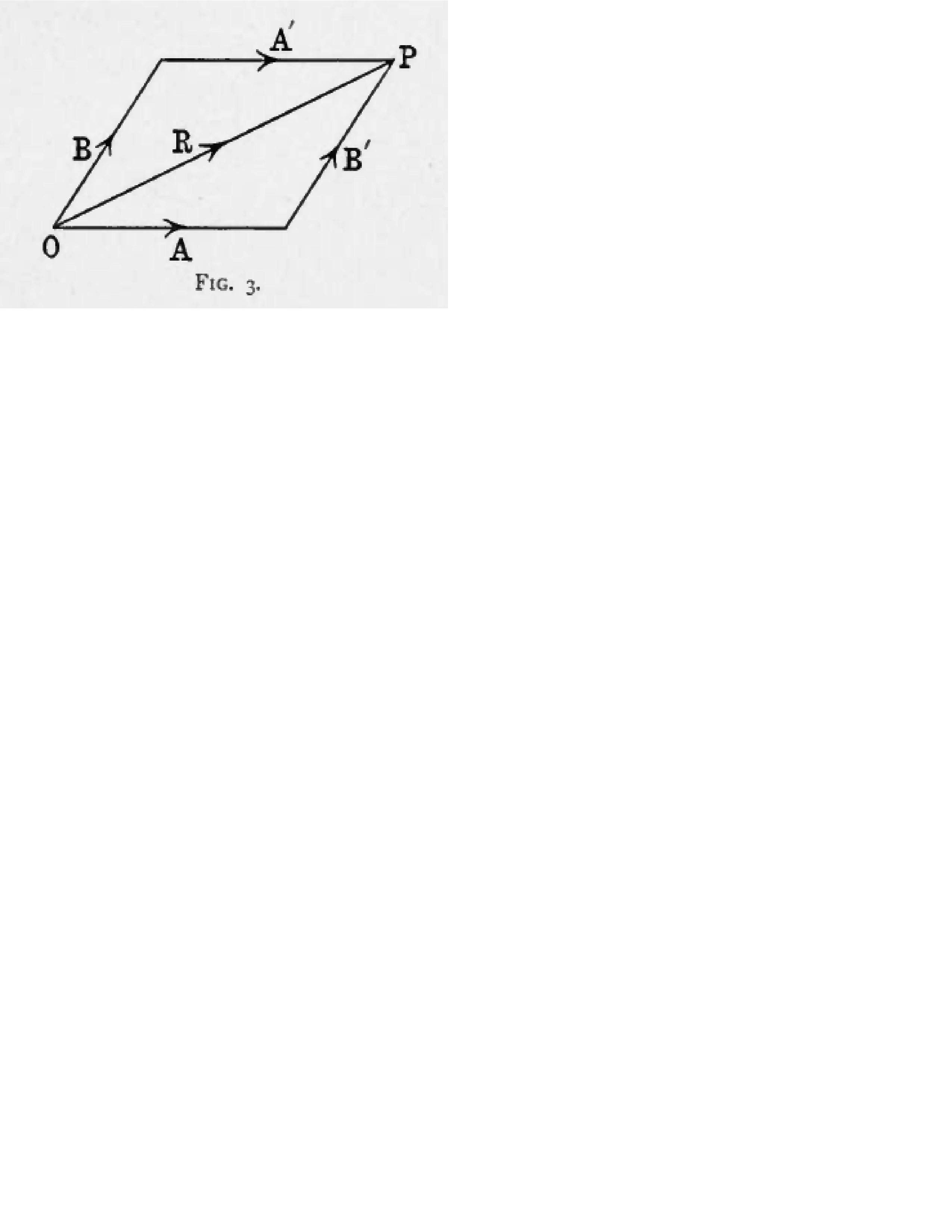
For the same reason we see that the sum of two vectors A, B starting from the same origin O is given by the diagonal OP of the parallelogram constructed on the addends A, B (Fig. 3). For, by Def. I., B′ = B, since B′ = B and B||B (i.e. B′ parallel to and concurrent with B), in Euclidean space, of course.

Again, in the same parallelogram, A′ = A (since A′ = A and A||A), and therefore

hence, for any two vectors,

Now, the sum of two vectors being again a vector, A + B = R, we can add to R any third vector, thus getting

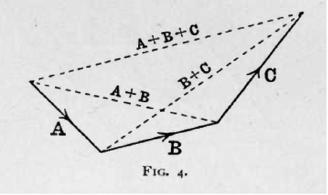
Again, arranging A, B, C in a chain, i.e. so that the end of A is the beginning of B, the end of B the beginning of C, we see at once (Fig. 4) that

the result being always the same, namely to get from the beginning of A to the end of C. The same thing is true for the sum of four, five and more vectors. Thus we get the following theorem:

Theorem I. The addition of vectors is commutative and associative, i.e. neither the order nor the grouping of the addends has an influence on the sum of any number of vectors.

Thus, the fundamental laws of ordinary algebraic summation of scalars hold good for vectors, without any reservation whatever.

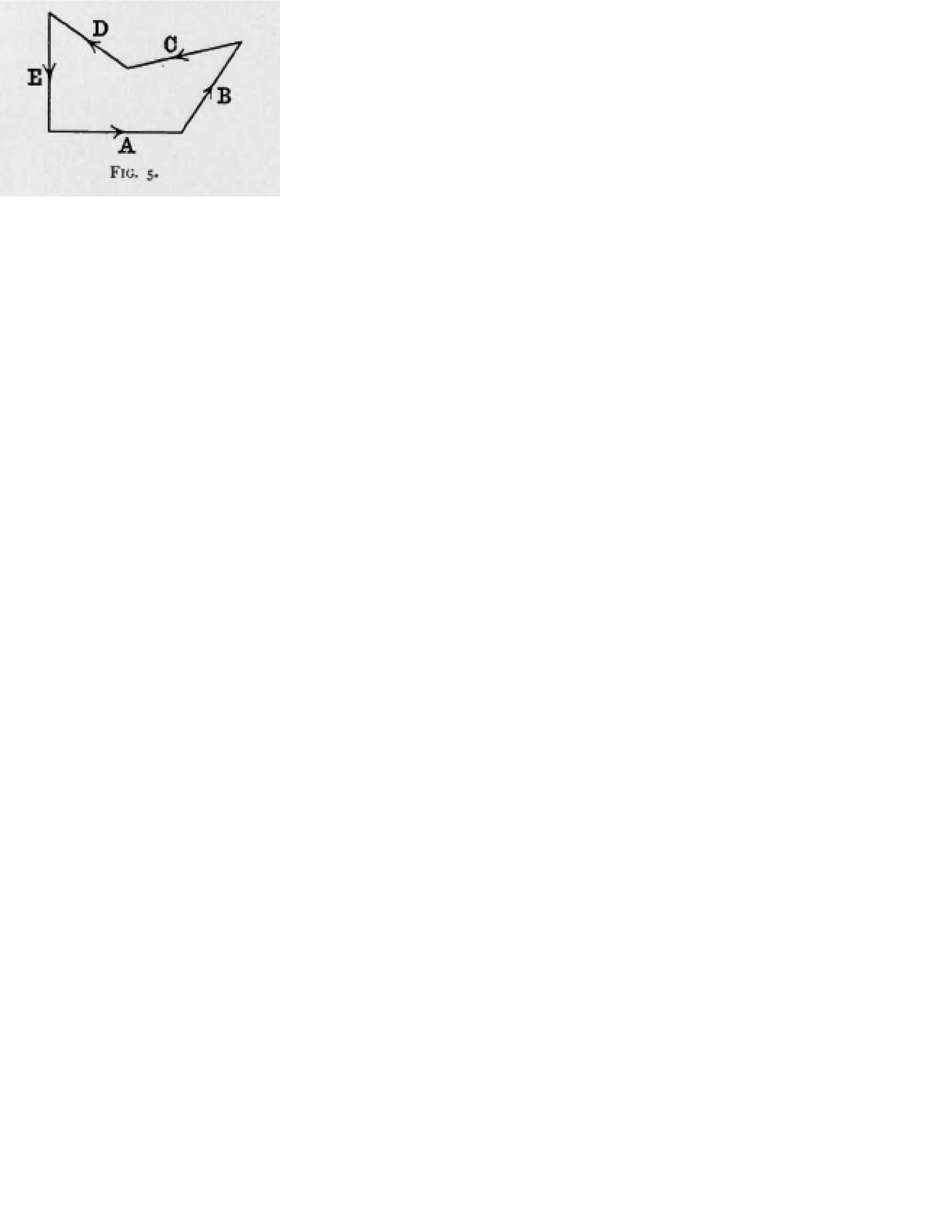
If, in a chain-like arrangement of any number of vectors, the end of the last coincides with the beginning of the first vector, then the sum of all these vectors is nil. Thus, in Fig. 5,

A vector is nil or zero, R = 0, if its tensor vanishes, R = 0. In fact, this remark is scarcely necessary.

The sum of any number of vectors having the same direction (i.e. of vectors parallel and of the same sense) is a vector of the same direction. In this particular case the tensor of the sum is equal to the sum of the tensors. Thus, the common sum is a particular case of the vector-sum.

Now, let us take the case of two or more equal vectors; then we see at once that

is a vector of the same direction as A but of twice its tensor, i.e. 2A, and that analogous properties belong to 3A, 4A, and so on. Again, understanding by A, A, etc., vectors which, repeated 2, 3, etc., times (as addends), give the vector A, and recurring to the generally known limit-reasoning, we obtain the meaning of

where n is any real positive scalar number, whole, fractional or irrational. Thus, nA will be a vector which has the same direction as A and the tensor of which is nA. In other terms, nA will be the vector A stretched in the ratio n : 1.

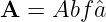
Thus, if bfâ be a unit-vector having the direction of A, remembering the definition of tensor, we may write

Any vector A may be represented in this way. Now A is one scalar, and bfâ implies two scalars, for instance the angles 𝜃, 𝜖; thus we see again that any vector implies 1 + 2 = 3 scalars.

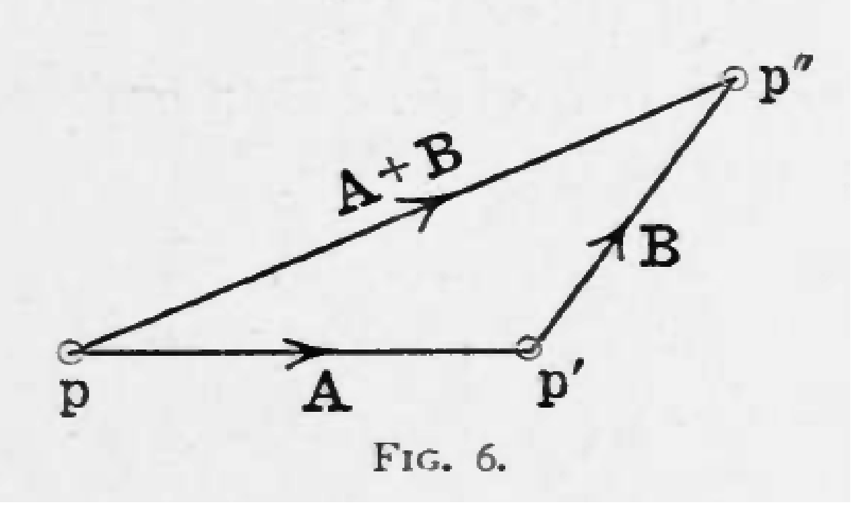
The addition of two (or more) vectors may be illustrated most simply by regarding them as defining translations in space of, say, a material particle. The translation A carries the particle from p to p′ (Fig. 6), the subsequent translation B carries it from p′ to p′′.

The result of A followed by B, or of B followed by A, i.e. A + B or B + A, is to carry the particle from p to p′′. Similarly, if A, B be velocities of translation, A + B will be the resultant velocity. The same applies to angular velocities, to accelerations or forces. If A, B denote two forces acting simultaneously on a material particle, A + B will be the resultant force acting on that particle.

more to come soon...