Wave Equations in Two and Three Dimensions and Spherical Waves

(Topic)

Wave Equations in Two and Three Dimensions and Spherical Waves

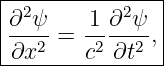
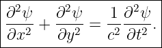
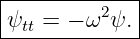
The one-dimensional wave equation,

|-2---------2--| |∂-ψ-= 1-∂-ψ-,| -∂x2----c2-∂t2--

(1)

describes waves whose spatial variation is restricted to one coordinate.

Real waves usually spread through two or three dimensions.

A vibrating membrane varies over two spatial coordinates.

Sound in open space varies over three.

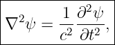
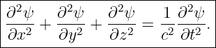
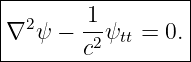
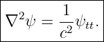
The natural multidimensional generalization is

|--------------| | 2 1 ∂2ψ | ∇ ψ = -2---2 , --------c--∂t---

(2)

where

2 ∇

(3)

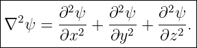
is the Laplacian.

This article develops:

the wave equation in two and three dimensions,
plane waves and the wave vector,
wavefronts as surfaces of constant phase,
exact spherically symmetric solutions,
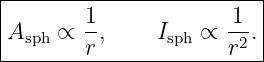
the 1∕r falloff of spherical-wave amplitude,
the 1∕r² falloff of spherical-wave intensity,
the contrast between cylindrical and spherical spreading.

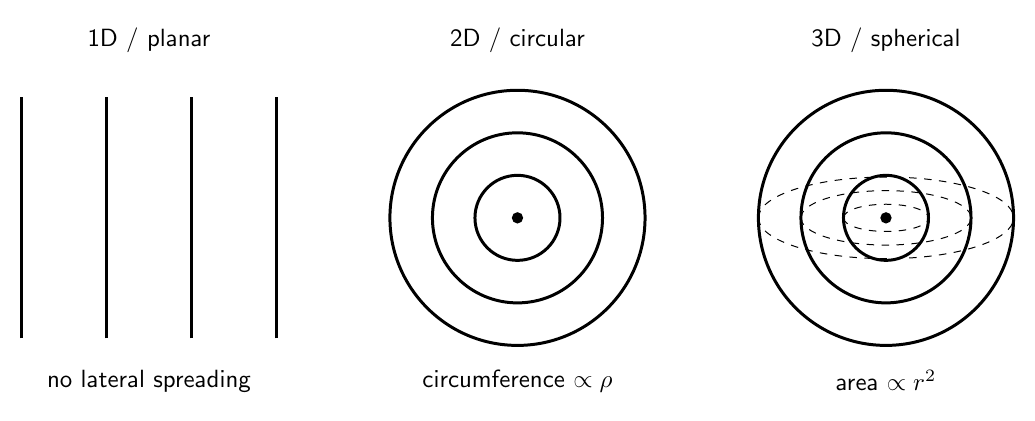
Figure 1. Idealized wavefront geometry in one, two, and three spatial dimensions. Planar propagation has no geometric spreading, circular spreading enlarges a circumference, and spherical spreading enlarges a surface area.

1 The Laplacian

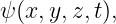
For a scalar field

ψ(x, y,z,t),

(4)

the Cartesian Laplacian is

|--------------------------| | 2 ∂2ψ- ∂2ψ- ∂2ψ- | |∇ ψ = ∂x2 + ∂y2 + ∂z2 .| ----------------------------

(5)

The Laplacian measures local spatial curvature.

In one dimension, only the first term remains.

Thus the one-dimensional wave equation is simply the one-coordinate version of the multidimensional equation.

2 Two-dimensional wave equation

If the field depends on

x, y,

(6)

but not on

z,

(7)

then

2 ∂--ψ ∂z2 = 0.

(8)

The wave equation becomes

|----------------------| |∂2ψ ∂2ψ 1 ∂2ψ | |---2 + ---2 = -2 --2-.| -∂x-----∂y-----c--∂t---

(9)

Examples include:

ideal transverse waves on a membrane,
approximately two-dimensional water-wave models,
scalar field models invariant along one axis.

3 Three-dimensional wave equation

In three dimensions,

|----------------------------| |∂2ψ ∂2ψ ∂2ψ 1 ∂2ψ | |--2-+ --2-+ --2-= -2---2 . -∂x-----∂y-----∂z-----c--∂t---

(10)

Equivalently,

|------------------| |∇2 ψ − 1-ψ = 0. | ---------c2--tt-----|

(11)

This scalar equation appears in:

acoustics,
elastic-wave approximations,
electromagnetic scalar components in suitable settings,
mathematical models of many other linear wave systems.

4 Plane-wave trial solution

Consider

|------------------------------| |ψ(r,t) = A cos(k ⋅ r − ωt + ϕ). --------------------------------

(12)

Here:

r is the position vector,
k is the wave vector,
ω is angular frequency,
ϕ is constant phase.

The magnitude of the wave vector is

|--------| |k = |k|.| ---------

(13)

Its direction is the direction of phase propagation.

5 Testing the plane wave

Let

Θ = k ⋅ r − ωt + ϕ.

(14)

For the trial solution,

ψ = A cosΘ.

(15)

Each spatial derivative produces a component of

k.

(16)

Therefore

|--------------| |∇2 ψ = − k2ψ. | ---------------

(17)

The second time derivative is

|------------| |ψ = − ω2ψ. | --tt----------

(18)

Substitution into the wave equation gives

2 ω2- − k ψ = − c2 ψ.

(19)

Thus

|-------| ω-=--ck-|

(20)

for the positive-frequency branch.

This is the nondispersive relation already encountered in one-dimensional wave propagation.

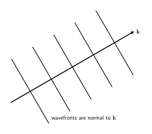
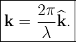
Figure 2. The wave vector k points Normal to planes of constant phase. Its magnitude is k = 2π∕λ.

6 Wave vector and wavelength

For a plane wave,

|--------| | 2π- | |k = λ .| ----------

(21)

The unit propagation direction is

|-------| ^ k- | k = k. | ---------

(22)

Therefore

|----------| |k = 2π^k. | ------λ----|

(23)

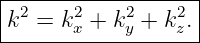
In Cartesian components,

|------------------------| |k = k e + k e + k e .| -------x-x----y-y----z-z-

(24)

Its magnitude satisfies

|-2----2----2----2-| -k--=-kx-+-ky +-kz.-

(25)

7 Surfaces of constant phase

For a plane wave, constant phase means

k ⋅ r − ωt + ϕ = constant.

(26)

At fixed time,

k ⋅ r = constant.

(27)

This is the equation of a plane perpendicular to

k.

(28)

Therefore plane-wave wavefronts are planes.

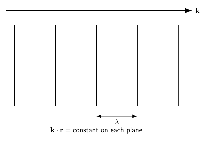
Figure 3. Parallel planes of constant phase move in the direction of k. Adjacent equal-phase planes are separated by one wavelength.

8 Example 1: a three-dimensional plane wave

Let

k = 3ex + 4ey m −1.

(29)

Then

k	=	(30)
	= 5 m⁻¹.	(31)

The wavelength is

λ	=	(32)
	=	(33)
	≈ 1.257 m.	(34)

c = 343 m ∕s,

(35)

then

ω = ck = 1715 rad∕s.

(36)

Thus

f	=	(37)
	≈ 272.95 Hz.	(38)

9 Why geometry changes amplitude

A plane wave can idealize propagation with no lateral spreading.

A point-like source in open three-dimensional space is different.

As energy propagates outward, it is distributed over larger spherical surfaces.

If the source emits constant time-averaged power

P,

(39)

that same power must cross every sphere centered on the source in a lossless medium.

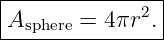
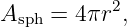
The area of a sphere is

|--------------| Asphere = 4πr2.| ----------------

(40)

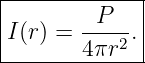
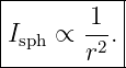
Therefore the average radial intensity is

|------------| | P | I (r) = ---2.| --------4πr---

(41)

This inverse-square law is a consequence of geometry.

10 Spherical symmetry

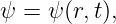
Suppose the field is spherically symmetric.

Then

ψ = ψ(r,t),

(42)

where

∘ ------------ r = x2 + y2 + z2.

(43)

There is no dependence on angular coordinates.

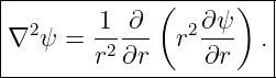
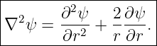
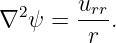
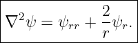
For such a field, the three-dimensional Laplacian reduces to

|-----------------------| | 1 ∂ ( ∂ψ ) | ∇2 ψ = -2--- r2--- . | --------r-∂r-----∂r-----

(44)

Expanding,

|--------------------| | 2 ∂2ψ 2 ∂ψ | |∇ ψ = ---2 + -----.| ---------∂r----r-∂r---

(45)

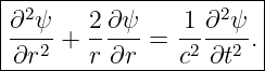
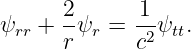
Therefore the radial three-dimensional wave equation is

|----------------------| |∂2ψ- 2∂-ψ 1-∂2ψ- | |∂r2 + r ∂r = c2∂t2 .| ------------------------

(46)

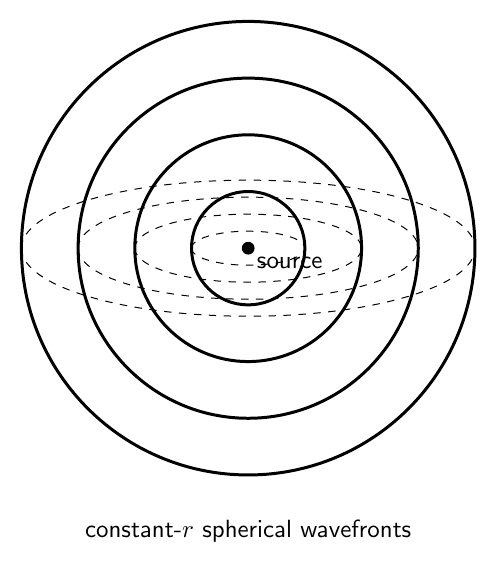
Figure 4. A spherically symmetric disturbance has constant field value over concentric spherical wavefronts. The wavefront area grows as 4πr².

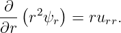
11 Reducing the radial equation

The radial equation contains the extra geometric term

2ψ . r r

(47)

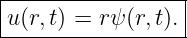
Introduce

------------------ | | u-(r,t)-=-rψ-(r,t).-

(48)

Equivalently,

ψ = u. r

(49)

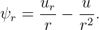
Differentiate with respect to

r.

(50)

First,

ur- u- ψr = r − r2.

(51)

Then

2 r ψr = rur − u.

(52)

Differentiate again:

∂ ( ) --- r2ψr = rurr. ∂r

(53)

Therefore

∇2 ψ = urr. r

(54)

Also,

ψ = utt. tt r

(55)

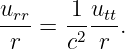
The radial wave equation becomes

urr= 1-utt. r c2 r

(56)

For

r > 0,

(57)

multiply by

r.

(58)

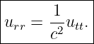
Then

|------------| | 1 | |urr = c2utt.| -------------

(59)

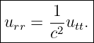
This is exactly the one-dimensional wave equation.

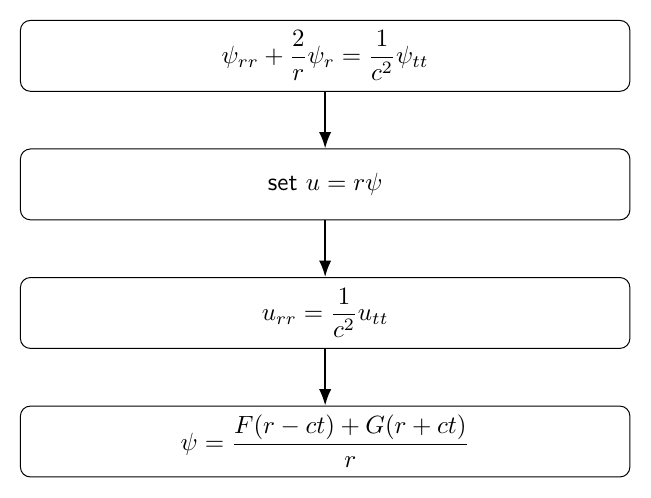
Figure 5. Multiplying the spherical field by radius removes the geometric-spreading term. The quantity u = rψ obeys the ordinary one-dimensional wave equation for r > 0.

12 General spherically symmetric solution

Because

u

(60)

satisfies the one-dimensional wave equation,

|------------------------------| u-(r,t)-=-F-(r −-ct)-+-G-(r +-ct).-

(61)

Therefore

|----------------------------------| |ψ(r,t) = 1F (r − ct) + 1-G (r + ct). ----------r------------r------------

(62)

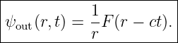
The first term is an outgoing spherical wave.

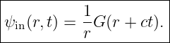
The second term is an incoming spherical wave.

Thus the exact radial propagation form in three dimensions contains a geometric

1∕r

(63)

amplitude factor.

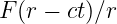
13 Outgoing spherical wave

An outgoing pulse has the form

|-----------1-----------| ψout(r,t) = -F (r − ct). | ------------r------------

(64)

The pulse shape in the variable

r − ct

(65)

translates outward at speed

c.

(66)

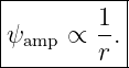
Its amplitude decreases as

|----------| | 1-| |ψamp ∝ r.| ------------

(67)

14 Incoming spherical wave

An incoming radial wave has

|----------------------| | 1 | |ψin(r,t) = --G (r + ct).| -----------r------------

(68)

Its constant-phase surfaces move toward decreasing

r.

(69)

In ideal mathematical models, incoming spherical waves focus toward the origin.

Real physical behavior near a source, scatterer, or focal region requires the actual boundary conditions there.

15 Harmonic spherical wave

Choose

F (r − ct) = A cos(k(r − ct) + ϕ).

(70)

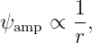
Since

ω = ck,

(71)

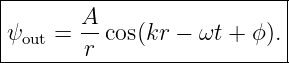
the outgoing field becomes

|----------------------------| ψ (r,t) = A-cos(kr − ωt + ϕ).| ----------r-------------------

(72)

The wavefronts are spheres satisfying

kr − ωt + ϕ = constant.

(73)

The phase propagates radially outward.

16 Amplitude and intensity spreading

For many linear wave systems, time-averaged intensity is proportional to the square of the field amplitude.

1- ψamp ∝ r,

(74)

then

|--------| | -1 | |I ∝ r2 .| ---------

(75)

This matches the power-conservation argument:

2 P = I(r)4πr = constant.

(76)

The amplitude law and inverse-square intensity law are therefore two expressions of the same geometric spreading.

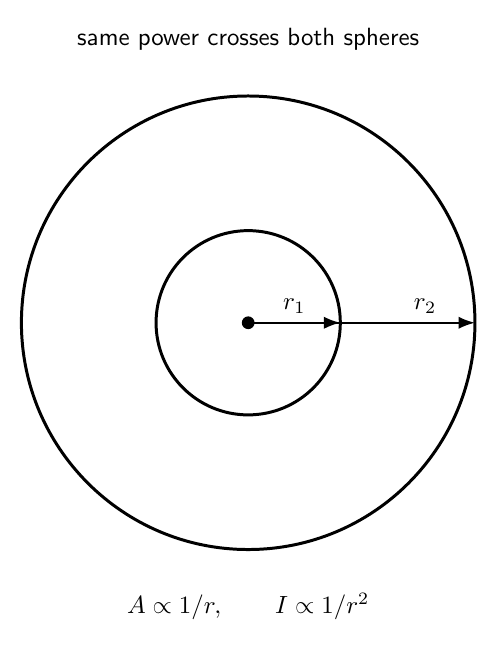
Figure 6. In lossless spherical spreading, the same power crosses successively larger spheres. Field amplitude scales as 1∕r while intensity scales as 1∕r².

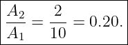
17 Example 2: amplitude ratio

Suppose a spherical-wave amplitude is

A1

(77)

at radius

r1 = 2.0m.

(78)

r2 = 10.0m,

(79)

the amplitude ratio is

A r --2 = -1 . A1 r2

(80)

Therefore

|----------------| |A2- 2-- | |A = 10 = 0.20.| --1---------------

(81)

The amplitude is one fifth as large.

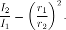
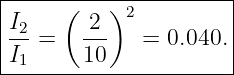
18 Example 3: intensity ratio

For the same radii,

I ( r )2 -2 = -1 . I1 r2

(82)

Thus

|----------------------| |I ( 2 )2 | |-2 = --- = 0.040. | -I1-----10-------------|

(83)

The intensity is one twenty-fifth as large.

19 Example 4: travel time

A spherical acoustic pulse travels from a source to radius

r = 1000 m

(84)

in air with

c = 343 m ∕s.

(85)

The travel time is

r t = c.

(86)

Therefore

t	=	(87)
	≈ 2.915 s.	(88)

20 Spherical acoustic pressure in the far field

For an acoustic point source sufficiently far from the source region, a harmonic pressure field often has the approximate form

|------------------------------| |p (r,t) = P0-cos(kr − ωt + ϕ).| --a--------r-------------------|

(89)

The associated average intensity decreases as

2 1∕r .

(90)

This is the spherical-wave counterpart of the plane-wave acoustics developed in M06-11.

Near the source, additional terms and source details can matter.

The simple

1∕r

(91)

form is most naturally interpreted as the radiating spherical-wave behavior away from the source region.

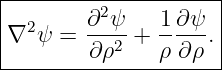
21 Two-dimensional radial spreading

Now consider a field depending only on the radial coordinate

ρ = ∘x2--+-y2-

(92)

in two dimensions.

For circular symmetry, the two-dimensional Laplacian becomes

|--------------------| | 2 ∂2ψ 1 ∂ψ | |∇ ψ = ---2 + -----.| --------∂-ρ----ρ-∂ρ---

(93)

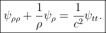
Therefore the radial two-dimensional wave equation is

|------------------| ψ + -1ψ = -1 ψ .| | ρρ ρ ρ c2 tt| --------------------

(94)

Notice the geometric term is now

1- ρψ ρ

(95)

rather than

2 rψr.

(96)

22 Cylindrical-wave spreading

For an ideal source uniform along one axis, wavefronts are cylindrical.

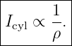
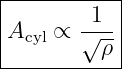
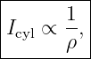
Power per unit source length spreads across a circumference proportional to

ρ.

(97)

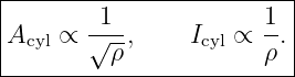
Therefore in the far field,

|--------| | 1 | Icyl ∝ ρ.| ----------

(98)

If intensity is proportional to amplitude squared, then

|----------| A ∝ 1√--| | cyl ρ | ------------

(99)

as a far-field scaling.

This differs from three-dimensional spherical spreading:

1 1 Asph ∝ -, Isph ∝ -2. r r

(100)

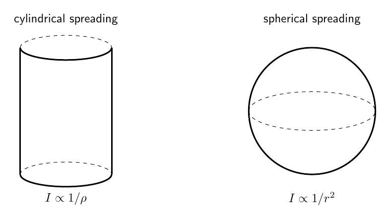
Figure 7. Geometric spreading depends on dimension. Ideal cylindrical wavefront area per unit length grows as ρ, while spherical area grows as r².

23 Why the two-dimensional radial solution is different

The substitution

u = r ψ

(101)

works exactly for spherical three-dimensional waves because the radial Laplacian contains the coefficient

2∕r.

(102)

The two-dimensional radial equation contains

1∕ρ.

(103)

It does not reduce to the same simple one-dimensional form through

u = √ ρ-ψ

(104)

without leaving an additional radial term.

Therefore

|--------------| | F (ρ − ct)| ψ ∝ ---√------| ----------ρ-----

(105)

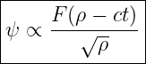
is best understood as a far-field cylindrical-wave scaling, not the exact arbitrary-pulse analogue of the three-dimensional

F (r − ct)∕r

(106)

solution.

24 Dimension and geometric spreading

The simplest geometric pattern is:

one-dimensional planar propagation: no geometric amplitude falloff,
two-dimensional cylindrical spreading: amplitude roughly 1∕ in the far field,
three-dimensional spherical spreading: amplitude exactly 1∕r for radial free waves away from the origin.

The corresponding intensity scalings are:

|-----------------| Iplane-∼-constant,--

(107)

|--------| Icyl ∝ 1,| -------ρ--

(108)

and

|----------| | 1- | -Isph-∝--r2.|

(109)

These are ideal lossless geometric scalings.

Real media can introduce absorption, scattering, boundaries, and refraction in addition to geometric spreading.

25 Energy conservation viewpoint

The spreading laws can be summarized through conservation of power.

For a plane wave crossing equal-area planes,

P = IA.

(110)

A

(111)

does not change, geometric spreading does not reduce

I.

(112)

For a cylindrical wave of source length

Lz,

(113)

the lateral area is

Acyl = 2πρLz.

(114)

Thus

I ∝ 1. ρ

(115)

For a spherical wave,

2 Asph = 4πr ,

(116)

I ∝ -1 . r2

(117)

26 Angular dependence in three dimensions

Not every three-dimensional wave is spherically symmetric.

In spherical coordinates,

ψ = ψ (r,𝜃,φ,t).

(118)

The full Laplacian contains radial and angular derivatives.

When variables are separated, the angular part leads to spherical harmonic functions.

The radial part then contains mode-dependent terms in addition to the basic radial derivatives.

The purely spherical case developed above is the angularly uniform mode.

It is often called the monopole angular pattern.

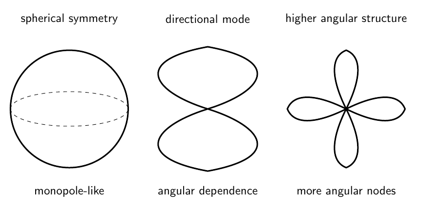
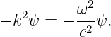
Figure 8. Spherical symmetry is only the angularly uniform case. More general three-dimensional waves can have directional angular structure, which is naturally organized into spherical-harmonic modes.

27 A preview of separation of variables

Suppose a three-dimensional harmonic wave is written as

ψ(r,t) = Φ (r )cos(ωt).

(119)

Substitution into the wave equation gives

|----------------| |∇2 Φ + k2Φ = 0,| -----------------

(120)

where

k = ω∕c.

(121)

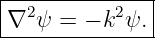
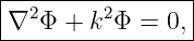
This is the Helmholtz equation.

It is the spatial equation underlying many standing-wave and scattering problems.

In rectangular geometry it leads to sine and cosine modes.

In cylindrical geometry it leads to Bessel functions.

In spherical geometry it leads to spherical Bessel functions and spherical harmonics.

Those methods are developed in later articles.

28 Outgoing-wave condition

In an unbounded region, a physical source generally produces waves carrying energy away from the source.

For spherical harmonic waves, the outgoing form is

|--------------------------| | A | ψout = --cos(kr − ωt + ϕ).| --------r-------------------

(122)

The incoming counterpart has the opposite radial phase propagation.

Boundary-value problems must specify which combination is physically appropriate.

For radiation from an isolated source, the outgoing-wave condition is the natural choice.

29 Near field and far field

The pure geometric

1∕r

(123)

radiating term describes the propagating spherical-wave part.

Near a physical source, other spatial dependencies can appear.

These near-field terms may decay faster with distance and can store energy locally rather than transport it steadily outward.

Far from a compact source, the radiating

1∕r

(124)

term dominates.

This is why the far-field intensity tends toward the inverse-square law.

30 Connection to Huygens construction

A propagating wavefront can be viewed geometrically as advancing normal to itself at speed

c

(125)

in a uniform isotropic medium.

Plane wavefronts remain plane.

Spherical wavefronts remain spherical.

The local direction of propagation is normal to the wavefront.

This geometric viewpoint connects:

the plane-wave vector k,
spherical radial propagation,
ray descriptions,
later diffraction and scattering ideas.

31 Common mistakes

Replacing the one-dimensional second derivative by only one Cartesian term in a genuinely multidimensional problem.
Forgetting that the Laplacian is the sum of second spatial derivatives in Cartesian coordinates.
Treating the wave vector as parallel to a plane wavefront rather than normal to it.
Confusing the magnitude k with one Cartesian component such as k_x.
Forgetting that k² = k_x² + k_y² + k_z².
Assuming a spherical wave has constant amplitude with distance.
Confusing 1∕r amplitude spreading with 1∕r² intensity spreading.
Applying the spherical 1∕r law to an ideal cylindrical source.
Treating F(ρ − ct)∕ as an exact arbitrary two-dimensional radial pulse.
Forgetting that the exact spherical radial reduction uses u = rψ.
Applying the radial spherical equation when the field has angular dependence.
Treating the origin r = 0 as an ordinary point of the F(r − ct)∕r formula without considering source or regularity conditions.
Confusing the wave equation with the time-independent Helmholtz equation.
Assuming every three-dimensional source is a monopole.
Attributing all amplitude loss to absorption when geometric spreading alone can reduce amplitude.

32 Practice exercises

Write the wave equation explicitly in two Cartesian dimensions.
Write the wave equation explicitly in three Cartesian dimensions.
Substitute a plane wave into the three-dimensional wave equation and derive ω = ck.
For a given vector k, calculate k, wavelength, and propagation direction.
Show that surfaces k ⋅ r = constant are planes normal to k.
Starting from the spherical radial Laplacian, derive $2 1 ψrr + --ψr = -2ψtt. r c$
Use u = rψ to reduce the spherical radial wave equation to the one-dimensional wave equation.
Derive the general incoming-plus-outgoing spherical solution.
Show that an outgoing harmonic spherical wave has amplitude proportional to 1∕r.
Derive the inverse-square intensity law from conservation of power through spheres.
Reproduce the amplitude and intensity ratio examples.
Derive the circularly symmetric two-dimensional radial wave equation.
Use power conservation to obtain the cylindrical far-field intensity scaling I ∝ 1∕ρ.
Explain why cylindrical amplitude scales approximately as 1∕ in the far field.
Explain how the Helmholtz equation arises from a time-harmonic wave equation.

33 Summary

The multidimensional scalar wave equation is

|--------1-----| |∇2 ψ = --ψtt.| ---------c2----|

(126)

A plane wave has the form

|--------------------------| |ψ = A cos(k ⋅ r − ωt + ϕ ), ---------------------------

(127)

with

|--------| -ω-=-ck.-|

(128)

For spherical symmetry,

|------------------| | 2 2- | |∇ ψ = ψrr + r ψr.| --------------------

(129)

The substitution

|-------| u = r ψ | ---------

(130)

reduces the radial three-dimensional wave equation to

|------------| | 1- | |urr = c2utt.| -------------

(131)

Therefore

|----------------------------------| | 1- 1- | |ψ(r,t) = rF (r − ct) + r G (r + ct). ------------------------------------

(132)

For an outgoing spherical wave,

|------------------------| |Asph ∝ 1, Isph ∝ 1-.| --------r-------------r2--

(133)

For an ideal cylindrical wave in the far field,

|------------------------| | 1 1 | Acyl ∝ √--, Icyl ∝ -.| ---------ρ-------------ρ--

(134)

The spatial geometry of a wave therefore controls how its amplitude and intensity spread even in a perfectly lossless medium.

References

[1] PhysicsLibrary, M06-11, Acoustic Waves, Sound Intensity, and Acoustic Impedance.

[2] PhysicsLibrary, M06-10, Fourier Analysis, Wave Packets, and Dispersion.

[3] PhysicsLibrary, M06-08, Continuous Strings, Standing Waves, and Normal Modes.

[4] A. P. French, Vibrations and Waves, W. W. Norton, 1971.

[5] G. B. Arfken, H. J. Weber, and F. E. Harris, Mathematical Methods for Physicists, 7th ed., Academic Press, 2013.

"Wave Equations in Two and Three Dimensions and Spherical Waves" is owned by bloftin.
(view preamble)

Wave Equations in Two and Three Dimensions and Spherical Waves