Damped Harmonic Motion
The ideal simple harmonic oscillator of M06-01 obeys
and oscillates forever.
Real oscillators lose mechanical energy.
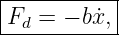
A standard model adds a resistive force proportional to velocity:
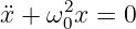
where
is the viscous damping coefficient.
For a mass attached to a spring,
Therefore
Dividing by
gives
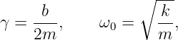
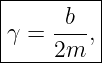
where
and
The parameter
sets the damping time scale.
The relation between
and
determines whether the system oscillates while decaying or returns to equilibrium without
oscillation.
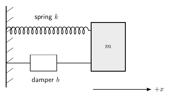
Figure 1. A damped spring-mass oscillator combines the restoring force −kx with a
velocity-dependent damping force −bẋ.
1 Viscous damping force
The damping force
opposes the instantaneous velocity.
Its dimensions are
Therefore
The damping rate
has the same dimensions as an angular frequency.
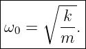
This allows a direct comparison between damping and the undamped natural frequency
2 State-space form
As in M06-01, define
Then
| ẋ = v, | | (19)
|
| v = −2γv − ω02x. | | (20) |
The complete state is still
In matrix form,
The damping regimes are therefore also eigenvalue regimes of this state matrix.
3 Characteristic equation
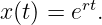
Seek a solution of the form
Then
Substitution into
gives
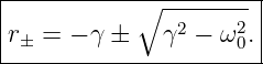
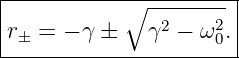
Thus
Everything depends on the sign of
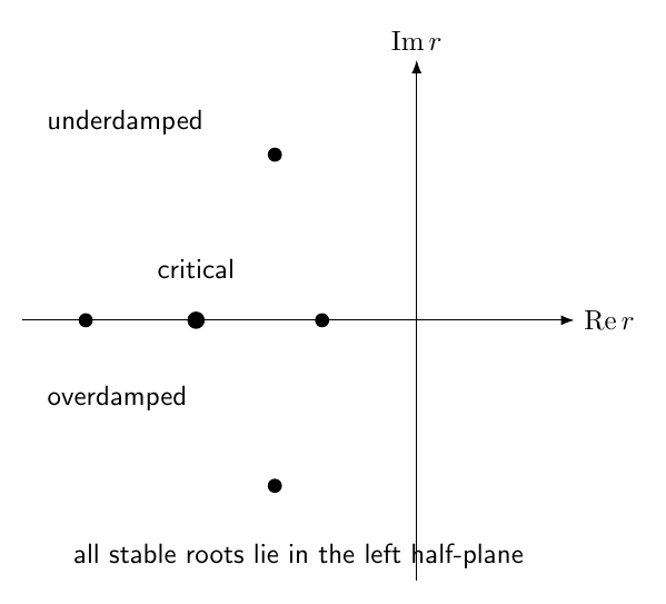
Figure 2. The damping regime is determined by the characteristic roots. Complex conjugate roots
produce decaying oscillation, a repeated real root gives critical damping, and two distinct
negative real roots give overdamping.
4 Damping ratio
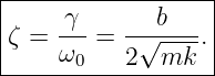
Define the dimensionless damping ratio
Then:
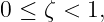
- underdamped:
- critically damped:
- overdamped:
The undamped limit is
5 Underdamped motion
If
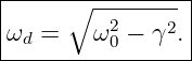
the roots are complex:
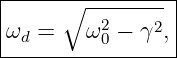
where
The real solution is
Equivalently,
The oscillation survives, but its envelope decays exponentially.
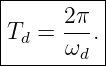
6 Damped period
The underdamped period is
Since
the damped period is slightly longer than the undamped period:
For weak damping,
the difference is small.
7 Underdamped initial-value solution
Let
Begin with
At
Differentiate:
| v(t) | = e−γt − γ(C cos ωdt + D sin ωdt) − γ(C cos ωdt + D sin ωdt) | (47)
|
| − Cωd sin ωdt + Dωd cos ωdt![]](https://images.physicslibrary.org/cache/objects/1490/make4ht/DampedHarmonicMotion45x.png) . . | (48) |
At
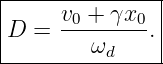
Thus
Therefore
8 Underdamped amplitude envelope
In amplitude-phase form,
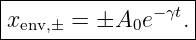
The positive and negative envelopes are
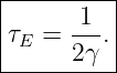
The amplitude envelope therefore has time constant
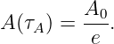
After one amplitude time constant,
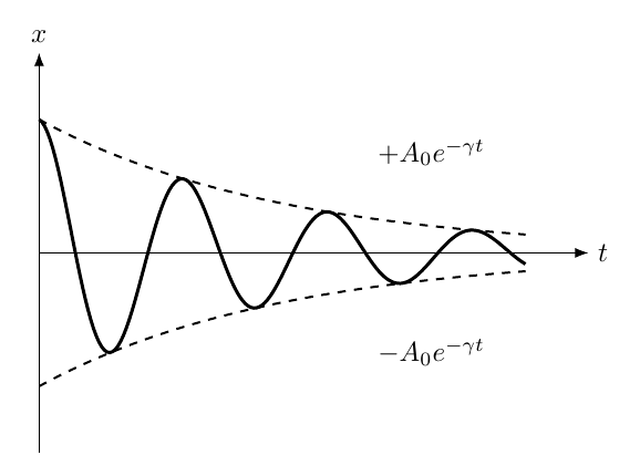
Figure 4. An underdamped oscillator remains sinusoidal while its amplitude is bounded by the
exponential envelopes ±A0e−γt.
9 Example 1: underdamped oscillator
Let
| m | = 1.0 kg, | (57)
|
| k | = 100 N∕m, | (58)
|
| b | = 4.0 kg∕s. | (59) |
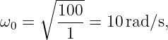
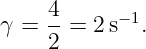
Then
and
Because
the motion is underdamped.
The damped angular frequency is
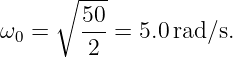
| ωd | = 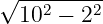 | (63)
|
| =  | (64)
|
| ≈ 9.80 rad∕s. | (65) |
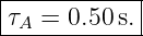
The amplitude time constant is
10 Critical damping
If
the characteristic equation has one repeated root:
A repeated root requires a second independent solution proportional to
Therefore
Critical damping separates oscillatory decay from nonoscillatory decay.
It is also the fastest possible return to equilibrium within this linear model without
oscillation.
11 Critical-damping initial-value solution
At
Differentiate:
At
Thus
Hence
12 Overdamped motion
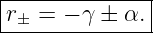
If
define
The two roots are real and negative:
Therefore
There is no sinusoidal oscillation.
One exponential mode decays slowly and the other rapidly.
At sufficiently long times, the slower mode dominates.
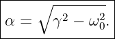
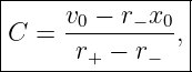
13 Overdamped initial-value solution
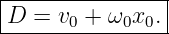
At
Also,
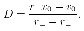
Solving,
and
These coefficients completely determine the overdamped trajectory.
14 The three regimes compared
The three forms are:
- underdamped:
- critically damped:
- overdamped:
All three return toward equilibrium when
Only the underdamped case crosses equilibrium repeatedly.
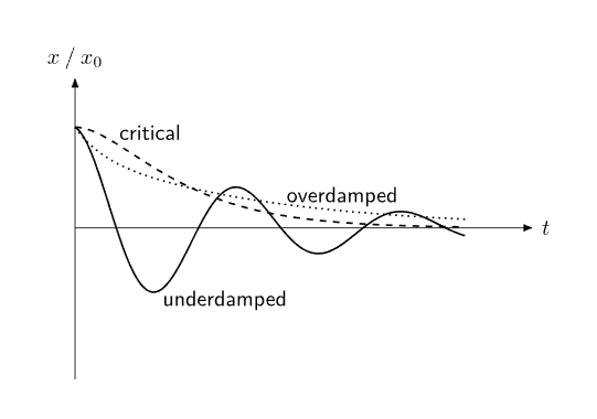
Figure 3. Underdamped motion oscillates through equilibrium, critical damping gives the fastest
nonoscillatory return, and overdamped motion returns more slowly as a sum of two decaying
exponentials.
15 Why critical damping is special
For a specified
and
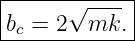
critical damping occurs when
If
the response oscillates.
If
the response is nonoscillatory but contains a slow exponential mode.
At
the system sits at the boundary and returns without oscillation as rapidly as possible in the linear
viscous model.
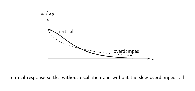
Figure 7. Critical damping lies at the boundary between oscillatory and overdamped behavior and
gives the fastest nonoscillatory return to equilibrium for the standard linear model.
16 Phase-plane behavior
The undamped SHO of M06-01 follows closed ellipses in the
phase plane.
Damping changes the geometry.
For the underdamped oscillator, the trajectory spirals toward
For critical and overdamped motion, trajectories approach the origin without repeated
revolutions.
Thus damping turns the equilibrium from a conservative center into an attracting equilibrium.
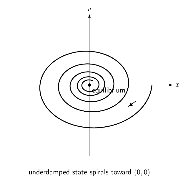
Figure 5. Damping causes phase-space trajectories to approach the equilibrium state (0,0).
Underdamped trajectories spiral inward, while critical and overdamped trajectories approach
without sustained rotation.
17 State-space eigenvalues and damping regimes
The state matrix is
Its eigenvalues satisfy
This gives
the same characteristic equation obtained from the scalar differential equation.
Therefore:
- complex conjugate eigenvalues correspond to a stable spiral,
- a repeated real eigenvalue corresponds to critical damping,
- two negative real eigenvalues correspond to a stable node.
This is the dynamical-systems interpretation of the three damping regimes.
18 Mechanical energy decreases
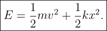
Define the usual mechanical energy
Differentiate:
 | = mvv + kxẋ | (103)
|
| = v(mẍ + kx). | (104) |
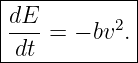
From the damped equation of motion,
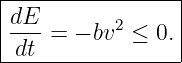
Therefore
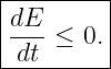
Since
Mechanical energy decreases monotonically.
The lost mechanical energy is transferred to thermal or other internal degrees of freedom
represented by the damping model.
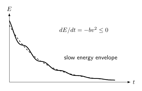
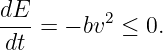
Figure 6. The viscous damping force removes mechanical energy at the instantaneous rate
dE∕dt = −bv2. Energy decreases most rapidly when speed is large.
19 Energy decay for light damping
For weak underdamping,
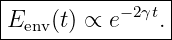
Because oscillator energy scales approximately with amplitude squared,
the slowly varying energy envelope obeys
Thus the characteristic energy-decay time is
The exact instantaneous mechanical energy contains oscillatory modulation.
The simple exponential statement refers to the slow envelope or cycle-averaged energy in the
lightly damped regime.
20 Logarithmic decrement
For an underdamped oscillator, consider two same-sign displacement maxima separated by one
damped period.
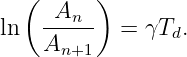
Their envelope amplitudes satisfy
Therefore
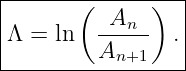
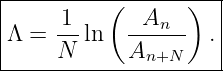
Define the logarithmic decrement:
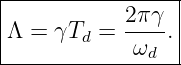
Then
More generally, using peaks
periods apart,
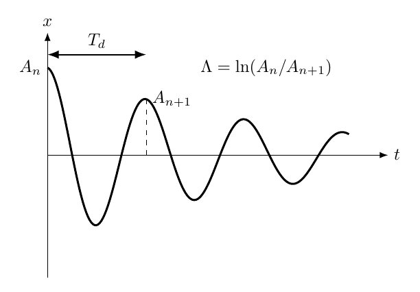
Figure 8. The logarithmic decrement measures damping from the ratio of successive same-sign
peak amplitudes in an underdamped free decay.
21 Example 2: damping from successive peaks
Suppose successive positive maxima are
and the damped period is
Then
| Λ | = ln  | (121)
|
| ≈ 0.2877. | (122) |
Thus
| γ | =  | (123)
|
| ≈ | (124)
|
| ≈ 0.575 s−1. | (125) |
22 Quality factor for weak damping
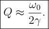
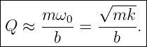
A common dimensionless measure of weak damping is the quality factor
Using
For light damping:
- large Q means slow decay,
- small Q means faster decay.
A more precise energy-based definition of
is especially useful for driven oscillators and Resonance and will be developed further in
M06-03.
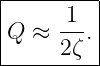
23 Relation between damping ratio and quality factor
For weak damping,
Therefore
This approximation is excellent when
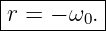
24 Example 3: classify from damping ratio
Let
Then
The critical damping coefficient is
| bc | = 2 | (135)
|
| = 2 | (136)
|
| = 20 kg∕s. | (137) |
Therefore:
- b = 8 kg/s is underdamped,
- b = 20 kg/s is critically damped,
- b = 30 kg/s is overdamped.
25 What damping does to frequency
For underdamped motion,
Thus damping reduces the oscillation frequency.
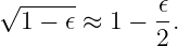
For weak damping, use
Then
| ωd | = ω0 | (140)
|
| ≈ ω0![[ ]
1-γ2-
1 − 2 ω2
0](https://images.physicslibrary.org/cache/objects/1490/make4ht/DampedHarmonicMotion130x.png) . . | (141) |
Therefore the frequency shift is second order in weak damping.
This is why lightly damped oscillators often oscillate at nearly the undamped natural frequency
even while their amplitude visibly decays.
26 Weak damping versus strong damping
A useful distinction is:
The word damped does not imply the motion is necessarily oscillatory.
27 The equilibrium state is an attractor
For
the origin
is an attracting equilibrium.
Mechanical energy satisfies
Therefore trajectories lose energy until they approach equilibrium.
This contrasts with the ideal SHO, whose phase-plane trajectories remain on closed
constant-energy ellipses.
28 Damping as a nonconservative process
The damping force is
Its instantaneous power is
This is always nonpositive.
The damping force therefore removes mechanical energy regardless of the sign of
The force reverses direction when the velocity reverses, but its power remains negative.
29 Example 4: instantaneous energy loss rate
Let
and suppose at one instant
Then
 | = −bv2 | (152)
|
| = −(3.0)(4.0) | (153)
|
| = −12 W. | (154) |
The negative sign means mechanical energy is being removed.
30 Critical damping and engineering design
Critical damping is important when oscillation is undesirable but rapid settling is needed.
Examples include idealized models of:
- door closers,
- measuring instruments,
- suspension components,
- actuator position control,
- vibration isolation systems.
Real devices can involve dry friction, nonlinear damping, hydraulic effects, or active
control.
The linear viscous model remains the fundamental first approximation.
31 Beyond viscous damping
Not all damping forces are proportional to velocity.
Examples include:
- Coulomb or dry friction,
- quadratic fluid drag,
- structural hysteresis,
- radiation damping,
- actively controlled damping.
For these systems, the equation
may be only an approximation.
The three classical damping regimes apply specifically to the linear viscous oscillator.
32 Common mistakes
- Assuming every damped oscillator is underdamped.
- Confusing the undamped natural frequency ω0 with the damped frequency ωd.
- Forgetting the factor of 2 in 2γ = b∕m.
- Writing γ = b∕m when using the equation ẍ + 2γẋ + ω02x = 0.
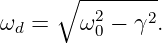
- Using ωd =
 instead of the minus sign.
- Forgetting the exponential envelope e−γt in the underdamped solution.
- Assuming the instantaneous mechanical energy is exactly proportional to e−2γt at every
instant.
- Saying critical damping returns to equilibrium faster than every underdamped
trajectory for every possible initial condition; the standard statement concerns fastest
nonoscillatory return in the linear model.
- Forgetting the te−ω0t term for a repeated characteristic root.
- Treating the overdamped solution as sinusoidal.
- Confusing damping ratio ζ with damping rate γ.
- Forgetting that logarithmic decrement uses same-sign peaks separated by a full damped
period.
- Forgetting that damping force always removes mechanical energy because Pd = −bv2.
- Assuming phase-space trajectories remain closed when damping is present.
- Applying viscous-damping formulas to dry-friction or quadratic-drag systems without
justification.
33 Practice exercises
- Derive the damped oscillator equation from the spring force and viscous damping force.
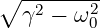
- Derive the characteristic roots r± = −γ ±
 .
.
- Express the damping ratio ζ in terms of m, b, and k.
- Derive the underdamped frequency ωd.
- Starting from x0 and v0, derive the underdamped initial-value solution.
- Derive the critical-damping solution and its initial-condition constants.
- Derive the overdamped initial-condition coefficients C and D.
- Show that the critical damping coefficient is bc = 2
 .
.
- Derive dE∕dt = −bv2.
- Explain why the underdamped phase-plane trajectory spirals toward equilibrium.
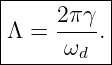
- Derive the logarithmic decrement formula Λ = 2πγ∕ωd.
- Use
two peaks separated by several cycles to derive the multi-cycle logarithmic-decrement
formula.
- Show that weak damping changes the oscillation frequency only at second order in
γ∕ω0.
- For m = 2 kg and k = 50 N/m, verify the critical damping coefficient in Example 3.
- Explain the dynamical-systems meaning of the eigenvalue transition from complex to
repeated real to distinct real roots.
34 Summary
The linearly damped harmonic oscillator obeys
With
The characteristic roots are
For
and the motion oscillates with exponentially decaying amplitude.
For
the system is critically damped.
For
it is overdamped.
Mechanical energy obeys
The underdamped logarithmic decrement is
Damping converts the closed phase-space orbits of the ideal oscillator into trajectories attracted
toward equilibrium.
M06-03 adds an external periodic force and develops driven motion, resonance, phase lag, and the
deeper role of the quality factor.
References
References
[1] PhysicsLibrary, M06-01, Simple Harmonic Motion.
[2] PhysicsLibrary, simple harmonic oscillator, canonical object
SimpleHarmonicOscillator.
[3] A. P. French, Vibrations and Waves, W. W. Norton, 1971.
[4] J. R. Taylor, Classical Mechanics, University Science Books, 2005.








![-force-- − 1
[b] = velocity = M T .](https://images.physicslibrary.org/cache/objects/1490/make4ht/DampedHarmonicMotion13x.png)
![[ ]
b- −1
m = T .](https://images.physicslibrary.org/cache/objects/1490/make4ht/DampedHarmonicMotion14x.png)


![|---[-]---[-----------]-[-]--|
| d x 0 1 x |
|-- v = − ω2 − 2γ v .|
-dt------------0-------------](https://images.physicslibrary.org/cache/objects/1490/make4ht/DampedHarmonicMotion19x.png)







![|--------−γt-----------------------|
-x(t) =-e---[C-cosωdt-+-D-sin-ωdt].|](https://images.physicslibrary.org/cache/objects/1490/make4ht/DampedHarmonicMotion34x.png)




![x(t) = e−γt[C cosω t + D sin ω t].
d d](https://images.physicslibrary.org/cache/objects/1490/make4ht/DampedHarmonicMotion41x.png)



![|-----------[---------------------------]--|
|x(t) = e−γt x0 cosωdt + v0-+-γx0-sin ωdt .|
----------------------------ωd-------------|](https://images.physicslibrary.org/cache/objects/1490/make4ht/DampedHarmonicMotion49x.png)








![v(t) = [D − ω0(C + Dt )]e−ω0t.](https://images.physicslibrary.org/cache/objects/1490/make4ht/DampedHarmonicMotion66x.png)


![|--------------------------−ω0t|
x-(t)-=-[x0 +-(v0 +-ω0x0-)t]e---.-](https://images.physicslibrary.org/cache/objects/1490/make4ht/DampedHarmonicMotion70x.png)













![[ ]
A = 0 2 1 .
− ω 0 − 2γ](https://images.physicslibrary.org/cache/objects/1490/make4ht/DampedHarmonicMotion92x.png)