
|
|
|
|||||||
with
In decibel form,
and a practical power budget is
Unless otherwise stated, the antennas are reciprocal, mutually far-field, polarization matched, and used in homogeneous free space. Gain values refer to the propagation directions of interest. Additional losses are power losses and are therefore subtracted in a dB link budget.
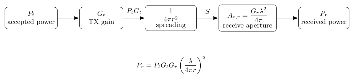
Figure. Friis can be read as a physical chain: accepted transmitter power is concentrated by transmit gain, spread over a sphere, and sampled by the receiver effective aperture.
Part I: Exercises
Exercise 1: Friis in linear unitsA transmitter delivers Pt = 2.00 W of accepted power to an antenna having directional gain Gt = 8.00. A receiving antenna 5.00 km away has directional gain Gr = 3.00. The frequency is 2.40 GHz. Find (a) wavelength, (b) received power in watts, (c) received power in dBW, and (d) received power in dBm.
Exercise 2: free-space path loss from first principlesFor an isotropic link at 915 MHz and range 3.00 km, calculate (a) wavelength, (b) the dimensionless free-space path loss, and (c) free-space path loss in dB. Verify the result using the engineering form
Exercise 3: distance scaling of path lossAt 2.40 GHz, calculate free-space path loss at 1.00 km, 2.00 km, and 10.0 km. From the results, verify that doubling distance adds approximately 6.02 dB of path loss and multiplying distance by ten adds 20 dB.
Exercise 4: frequency scaling at fixed antenna gainsAt a fixed range of 1.00 km, calculate free-space path loss at 1.00 GHz and 2.00 GHz. Explain why doubling frequency adds approximately 6.02 dB when the antenna gains are held fixed. Relate the result to the receive-aperture law
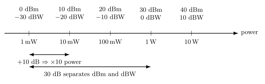
Figure. dBm and dBW are logarithmic absolute power units. A 10 dB increase multiplies power by ten, while dBm and dBW differ by exactly 30 dB.
Exercise 5: dB, dBm, dBW, and wattsConvert each quantity as requested:
Then state the distinction between a quantity expressed in dB and an absolute power expressed in dBm or dBW.
Exercise 6: a basic logarithmic link budgetA transmitter produces 30.0 dBm. The transmit feed line loses 1.50 dB, the transmitting antenna gain is 12.0 dBi, the receiving antenna gain is 8.00 dBi, and the receive feed line loses 2.00 dB. An additional 1.00 dB implementation loss is specified. The link operates at 5.80 GHz over 2.00 km. Find (a) free-space path loss and (b) received power after all listed losses, in dBm and watts.
Exercise 7: linear-polarization mismatchTwo linearly polarized antennas have polarization axes separated by 40.0∘. Find (a) the polarization loss factor, (b) polarization loss in dB, and (c) the received power if all other link effects would have produced −85.0 dBm under perfect polarization alignment.
Exercise 8: circular-to-linear polarization mismatchAn ideal circularly polarized wave is received by an ideal linearly polarized antenna. Find the polarization loss factor and polarization loss in dB. If the matched-polarization link prediction was −90.0 dBm, find the available power after this polarization mismatch alone.
Exercise 9: terminal mismatch lossAt the receiving antenna terminals, the magnitude of the reflection coefficient is
Find (a) the accepted-power fraction 1 −|ΓA|2, (b) mismatch loss in dB, and (c) delivered power if the available matched power would have been −80.0 dBm. Explain why the same mismatch loss must not be subtracted again if the receive antenna specification already uses realized gain.
Figure. A dB link budget is additive bookkeeping. Gains enter with positive signs; path, feed, atmospheric, polarization, pointing, and other losses enter with negative signs.
Exercise 10: complete microwave link budgetA 10.0 GHz point-to-point link spans 15.0 km. The transmitter output is 43.0 dBm. The transmit feed loss is 2.00 dB and transmit antenna gain is 18.0 dBi. The receive antenna gain is 25.0 dBi and receive feed loss is 1.50 dB. Include a 0.70 dB polarization loss, 1.20 dB atmospheric loss, and 1.00 dB pointing loss. Calculate (a) free-space path loss, (b) received power in dBm, and (c) received power in watts.
Exercise 11: maximum range from a receiver thresholdA 2.40 GHz radio transmits 20.0 dBm. Its transmit feed loss is 1.00 dB, transmit antenna gain is 5.00 dBi, receive antenna gain is 2.00 dBi, and all other losses total 3.00 dB. The receiver threshold is −100 dBm. Neglect fading margin. Determine (a) the maximum allowable free-space path loss and (b) the corresponding free-space range.
Exercise 12: field-strength and Friis cross-checkA transmitter has EIRP 100 W. At r = 1.00 km, a receiving antenna operates at 900 MHz and has gain 6.00 dBi toward the transmitter. Using
and
find (a) incident power density, (b) RMS electric-field magnitude, (c) receive effective aperture, and (d) received power. Verify the same received power directly from Friis using PtGt = EIRP.
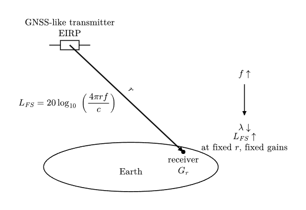
Figure. A GNSS-style link is an extreme-range Friis problem. At fixed range and fixed antenna gains, the higher-frequency signal has greater free-space path loss because fixed gain corresponds to smaller effective aperture as wavelength decreases.
Exercise 13: GNSS-style received carrier powerConsider an intentionally simplified GPS-L1-like link with
Assume transmitter EIRP 27.0 dBW in the receiver direction, receive gain 0 dBi, and 2.00 dB of additional propagation and implementation loss. Find (a) free-space path loss, and (b) received carrier power in dBW, dBm, and watts. This is a link-budget exercise, not a specification for a particular GNSS satellite or receiver.
Exercise 14: GNSS-style link with receive gain and polarization lossUse the same L1 frequency and range as Exercise 13, but now let the transmitter EIRP be 26.5 dBW, receive antenna gain be 3.00 dBi, polarization loss be 1.50 dB, and all other losses total 1.00 dB. Find the received power in dBW, dBm, and watts. Identify which terms are transmitter-side, propagation-side, and receiver-side.
Exercise 15: compare L1-like and L5-like path lossAt the same 20,200 km range, compare the ideal free-space path loss at
and
Find the path-loss difference in dB and the corresponding linear power ratio for links having the same EIRP and the same receive gain. Explain why this comparison assumes fixed gain rather than fixed physical receive aperture.
Exercise 16: Julia sweep of free-space link behaviorWrite a Julia program that
State the expected logarithmic slopes before writing the code.
Part II: Complete Worked Solutions
Solution 1: Friis in linear unitsThe wavelength is
Friis gives
Therefore
In dBW,
Since
we obtain
Solution 2: free-space path loss from first principlesAt 915 MHz,
Then
Thus
In decibels,
The engineering form gives
with the small last-digit difference determined by the rounded constant 32.45.
Solution 3: distance scaling of path lossAt 2.40 GHz,
Therefore doubling range changes the loss by
and multiplying range by ten changes it by
This follows directly from
Solution 4: frequency scaling at fixed antenna gainsAt r = 1.00 km,
The difference is
The same result follows from
At fixed receive gain,
Thus a gain-normalized receiving antenna has one-quarter the effective aperture when frequency doubles, corresponding to 6.02 dB less received power. This does not mean that ideal free space absorbs more energy at high frequency.
Solution 5: dB, dBm, dBW, and wattsFor dBm,
Therefore
Similarly,
For 5.00 W,
so
A value in dB is ordinarily a logarithmic ratio. dBm and dBW are absolute power levels because their reference powers are fixed at 1 mW and 1 W, respectively.
Solution 6: a basic logarithmic link budgetFirst calculate free-space path loss:
Now perform the power bookkeeping:
Converting to watts,
Thus
Solution 7: linear-polarization mismatchFor two linear polarizations separated by angle ψ,
At ψ = 40.0∘,
The polarization loss is
Therefore
Solution 8: circular-to-linear polarization mismatchAn ideal circularly polarized wave has equal average power in two orthogonal linear components. An ideal linear antenna selects one of those components, so
The loss is
Therefore the predicted receive power becomes
Solution 9: terminal mismatch lossThe fraction of available power accepted by the mismatched load is
Thus
The mismatch loss is
Therefore
If the antenna gain in the link budget is already a realized gain, mismatch has already been included in that gain definition. Subtracting Lmis again would double-count the same physical effect.
Solution 10: complete microwave link budgetThe free-space path loss is
The complete budget is
In watts,
Hence
Solution 11: maximum range from a receiver thresholdRearrange the link budget so the maximum allowable path loss is the remaining power margin:
Thus
From
solve for range:
At 2.40 GHz,
Therefore
A practical design would normally reserve additional fading, implementation, and environmental margin rather than operate exactly at this threshold.
Solution 12: field-strength and Friis cross-checkThe incident power density is
The RMS electric field is
At 900 MHz,
A gain of 6.00 dBi corresponds to
Hence
The receive power is
Now use Friis with PtGt = 100 W:
which gives the same 2.797 × 10⁻⁷ W. The field-strength, power-density, effective-aperture, and Friis descriptions are therefore mutually consistent.
Solution 13: GNSS-style received carrier powerFor f = 1.57542 GHz and r = 20,200 km,
The link budget is
Therefore
In watts,
The extremely small carrier power is why GNSS receiver analysis is normally expressed relative to noise spectral density rather than by received power alone.
Solution 14: GNSS-style link with receive gain and polarization lossThe L1 free-space path loss is unchanged:
The link budget is
Therefore
In watts,
Here 26.5 dBW is the transmitter-side EIRP. The 182.50 dB FSPL and 1.50 dB polarization term describe propagation/coupling effects. The 3.00 dBi receive gain is receiver-side directional collection. The final 1.00 dB term represents other specified implementation or propagation losses according to the chosen reference planes.
Solution 15: compare L1-like and L5-like path lossAt 20,200 km,
Thus
For otherwise identical links,
Thus, under the stated fixed-gain assumptions, the lower-frequency link has about 1.79 times the received power purely from the wavelength-dependent Friis factor. The fixed-gain qualification matters. If instead the same physical aperture were used efficiently at both frequencies, gain itself would scale approximately as 1∕λ2, and the apparent frequency dependence could change. Friis must always be interpreted together with how the antennas are being held fixed.
Solution 16: Julia sweep of free-space link behaviorBecause
the expected slope is 20 dB per decade in either range or frequency when the other variables and antenna gains are fixed. One Julia implementation is:
using Printf

const c = 299_792_458.0

fspl_db(r, f) = 20*log10(4*pi*r*f/c)
received_dbm(pt_dbm, gt_dbi, gr_dbi, r, f, loss_db=0.0) =
    pt_dbm + gt_dbi + gr_dbi - fspl_db(r,f) - loss_db

freq = 10 .^ range(log10(100e6), log10(10e9), length=201)
ranges = [1e3, 10e3, 100e3]

for r in ranges
    vals = fspl_db.(r, freq)
    @printf("r = %.0f km: FSPL %.2f to %.2f dB\n",
            r/1e3, vals[1], vals[end])
end

# Verify decade scaling.
f0 = 1.0e9
@printf("range decade change = %.6f dB\n",
        fspl_db(10e3,f0) - fspl_db(1e3,f0))
@printf("frequency decade change = %.6f dB\n",
        fspl_db(1e3,10e9) - fspl_db(1e3,1e9))

# Example user-defined link.
pt_dbm = 30.0
gt_dbi = 8.0
gr_dbi = 3.0
loss_db = 2.0
r = 5e3
f = 2.4e9
pr_dbm = received_dbm(pt_dbm,gt_dbi,gr_dbi,r,f,loss_db)
@printf("example Pr = %.3f dBm\n", pr_dbm)

# Simplified GNSS-style Exercise 13.
f_l1 = 1.57542e9
r_gnss = 20_200e3
eirp_dbw = 27.0


other_loss_db = 2.0
lfs = fspl_db(r_gnss,f_l1)
pr_dbw = eirp_dbw - lfs - other_loss_db
@printf("GNSS-style FSPL = %.3f dB\n", lfs)
@printf("GNSS-style Pr = %.3f dBW = %.3f dBm\n",
        pr_dbw, pr_dbw + 30)
The expected checks are approximately
and
For the simplified L1-like case, the script should reproduce approximately
and
What EM25E1 adds to the seriesEM25 derived the Friis equation and free-space path loss from electromagnetic power density and receive effective aperture. EM25E1 makes that theory operational. The worked problems connect linear power, logarithmic units, polarization and mismatch factors, practical loss bookkeeping, inverse range calculations, field strength, and satellite-scale received powers in one consistent reference-plane framework. The calculation chain is
The next article can therefore introduce thermal-noise power and spectral density,
so that the received carrier power obtained here can be converted into C∕N0.
References
[1] Harald T. Friis, “A Note on a Simple Transmission Formula,” Proceedings of the IRE, vol. 34, no. 5, pp. 254–256, 1946. [2] Constantine A. Balanis, Antenna Theory: Analysis and Design, 4th ed., Wiley, 2016. [3] Warren L. Stutzman and Gary A. Thiele, Antenna Theory and Design, 3rd ed., Wiley, 2012. [4] David M. Pozar, Microwave Engineering, 4th ed., Wiley, 2012. [5] Elliott D. Kaplan and Christopher J. Hegarty, eds., Understanding GPS/GNSS: Principles and Applications, 3rd ed., Artech House, 2017. "Electromagnetic Waves, Antennas, and RF: Friis Transmission Equation, Free-Space Path Loss, and RF Link Budgets - Exercises" is owned by bloftin.
This object's parent. Cross-references: electric field, average power, linear polarizations, energy, program, effective aperture, realized gain, magnitude, polarization loss factor, antenna gains, free-space path loss, relation, EM26, impedance, units, Power, Friis transmission equation, EM25 This is version 1 of Electromagnetic Waves, Antennas, and RF: Friis Transmission Equation, Free-Space Path Loss, and RF Link Budgets - Exercises, born on 2026-10-10. Object id is 1456, canonical name is ElectromagneticWavesAntennasAndRFFriisTransmissionEquationFreeSpacePathLossAndRFLinkBudgetsExercises. Accessed 7 times total. Classification:
|
|
|
|
Pending Errata and AddendaNone.
|
DiscussionNo messages.
|
Interact |
![[parent]](https://images.physicslibrary.org/images/uparrow.png)










 10
10


