Electromagnetic Waves, Antennas, and RF: Transmission Lines and the Telegrapher’s
Equations
EM21 showed that a traveling electromagnetic wave reflects whenever it encounters an impedance
discontinuity. Transmission-line theory is the one-dimensional distributed version of the same
physics. Instead of describing the fields everywhere in the cross-section, we describe the line by a
voltage v(z,t) and current i(z,t) that vary with both position and time. The result is not a lumped
circuit in the ordinary low-frequency sense: it is a wave system governed by partial differential
equations [1, 2, 3, 4].
The central chain developed here is
The algebra will strongly resemble EM21. That is not an accident. A material boundary and a
transmission-line load are both wave-impedance discontinuities.
1 Why a wire becomes a wave problem
At sufficiently low frequency, a short connection can often be approximated as an ideal wire:
voltage is taken to be the same everywhere along it, and current changes everywhere essentially at
once. That approximation fails when the physical length becomes a significant fraction
of a wavelength or when the signal rise time becomes comparable to the propagation
delay.
A transmission line is therefore modeled as a distributed electromagnetic system. Over a
small segment dz, four per-unit-length parameters summarize the local field storage and
loss:
| R | [Ω∕m] | | series conductor resistance, | (2)
|
| L | [H∕m] | | series magnetic-energy storage, | (3)
|
| G | [S∕m] | | shunt dielectric leakage, | (4)
|
| C | [F∕m] | | shunt electric-energy storage. | (5) |
The parameters L and C are especially important physically. A propagating line wave continuously
exchanges energy between electric-field storage and magnetic-field storage, just as the plane waves
of EM16–EM20 do. The parameters R and G dissipate part of that energy into Conductor and
dielectric loss.
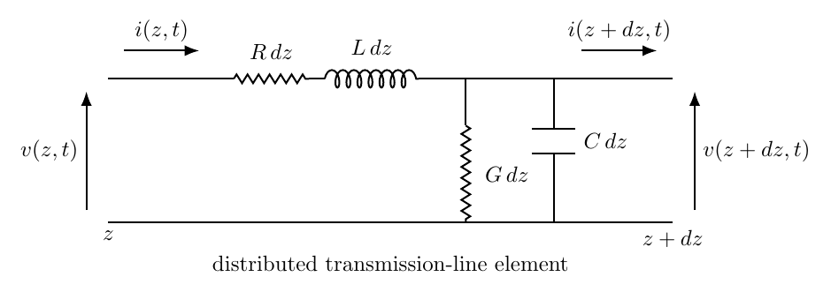
Figure. Differential transmission-line element. The series terms Rdz and Ldz act along
the conductors, while Gdz and C dz connect the two conductors.
2 Deriving the first telegrapher equation
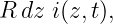
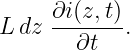
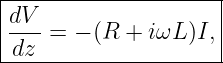
Consider the small line segment from z to z + dz. Apply Kirchhoff’s voltage law around the series
path. The voltage drop across the resistance is
and the inductor drop is
Therefore
Expand the voltage at z + dz to first order:
Ignoring terms of order dz2 and higher gives
Divide by dz:
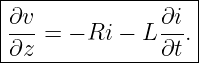
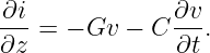
This is the first telegrapher equation. It says that spatial change of voltage is produced by both
resistive drop and time-varying magnetic energy storage.
3 Deriving the second telegrapher equation
Now apply current conservation to the same segment. The current entering at z differs from the
current leaving at z + dz because some current flows through the shunt conductance and
capacitance:
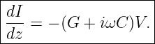
Using
gives
Together,
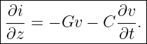
These are the time-domain telegrapher’s equations. They are coupled first-order partial differential
equations in space and time.
4 The full lossy wave equations
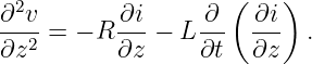
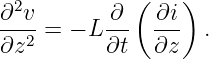
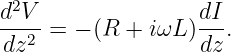
The first-order system can be combined into second-order equations. Differentiate the voltage
equation with respect to z:
Substitute
Then
 | = RGv + RC + LG + LG + LC + LC | (18)
|
| = RGv + (RC + LG) + LC + LC . . | (19) |
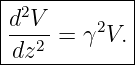
Therefore
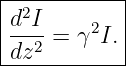
The current obeys the identical form:
The LC term produces wave propagation, the terms proportional to RC + LG produce first-order
damping, and RG is a loss-coupling term. This is the distributed-circuit counterpart of the damped
electromagnetic wave equation developed in EM20.
5 Lossless line: the wave equation appears immediately
Before moving to the full sinusoidal solution, consider the ideal lossless case
Then
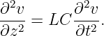
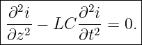
Differentiate the first equation with respect to z:
Substitute the second equation:
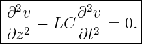
Hence
Similarly,
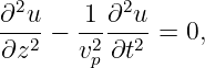
Comparing with the standard one-dimensional wave equation,
we identify
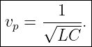
Thus the finite propagation speed of a transmission-line signal follows directly from the distributed
electric and magnetic energy storage.
6 Sinusoidal steady state and phasor form
Assume sinusoidal time dependence with the convention
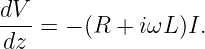
Then time differentiation becomes multiplication by iω, and the telegrapher equations reduce to
ordinary differential equations:
These equations show that the natural series impedance per unit length is
and the natural shunt admittance per unit length is
7 Deriving the propagation constant
Differentiate the voltage equation once more:
Using the current equation,
Define the propagation constant
Then
The same derivation gives
Exactly as in EM20,
is the attenuation constant and
is the phase constant.
8 Forward and backward traveling waves
The general voltage solution is
The first term propagates in the +z direction; the second propagates in the −z direction.
To obtain the current, substitute the voltage solution into
Differentiating gives
Therefore
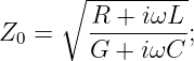
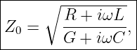
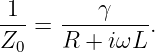
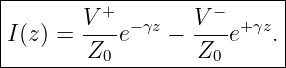
The ratio multiplying the traveling-wave voltage naturally defines the characteristic
impedance.
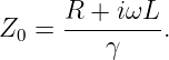
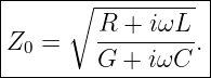
9 Deriving the characteristic impedance
For the forward wave,
From the preceding equation,
Hence
Using
we obtain
The complete current solution is therefore
The minus sign in the reflected current is crucial. The reflected wave transports energy toward
decreasing z, so its current direction is opposite to the reference direction chosen for the forward
wave.
10 Lossless-line results
For
the propagation constant becomes
| γ | = 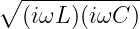 | (53)
|
| = iω . . | (54) |
Thus
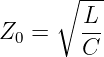
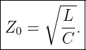
The characteristic impedance is purely real:
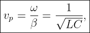
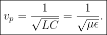
The phase velocity is
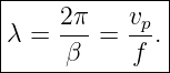
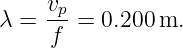
and the wavelength is
These relations reveal the physics of a line very cleanly: L and C together set the propagation
speed, while their ratio sets the wave impedance.
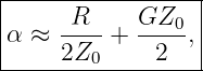
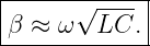
11 Low-loss approximation
Many practical RF lines satisfy
Expanding the exact propagation constant to first order in the small loss terms gives
where the Z0 on the right is approximately the lossless value  , while
The two contributions to α separate conductor loss and dielectric loss. The exact formulas should
be used when the low-loss inequalities are not satisfied.
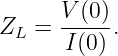
12 The load creates the reflected wave
Let the load be located at z = 0 and let the line extend toward negative z. The load impedance
is
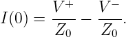
At the load,
while
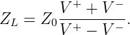
Thus
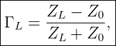
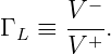
Define the voltage reflection coefficient at the load by
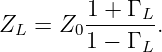
Then
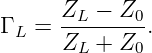
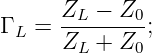
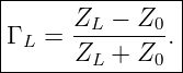
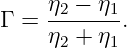
Solving for ΓL gives
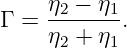
This is the transmission-line counterpart of the normal-incidence electromagnetic boundary result
from EM21,
The symbols are different, but the wave physics is the same.
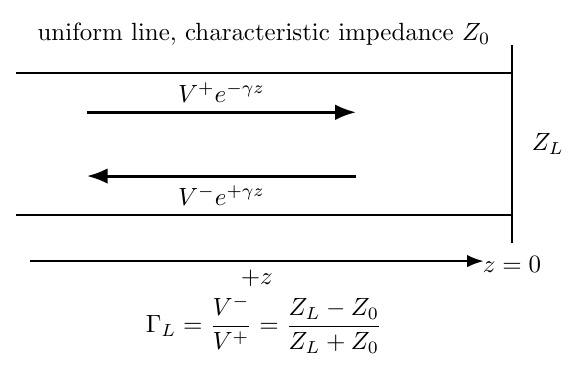
Figure. A load ZL generally produces a reflected wave. The characteristic impedance Z0 is
the voltage-to-current ratio of a single traveling wave, not the ordinary resistance of the
conductors.
13 Special load cases
Three cases should be recognized immediately.
13.1 Matched load
If
then
There is no reflected wave.
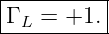
13.2 Open circuit
For
we obtain
The reflected voltage has the same phase as the incident voltage at the load, while the forward and
reflected currents cancel there.
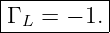
13.3 Short circuit
For
we obtain
The reflected voltage reverses phase so that the total load voltage vanishes.
14 Reflection coefficient away from the load
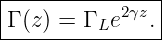
At an arbitrary position z, the ratio of reflected to incident voltage is
| Γ(z) | =  | (76)
|
| = ΓLe2γz. | (77) |
Therefore
For a lossless line,
so |Γ| is constant along the line while its phase rotates with position.
For a lossy line extending toward negative z, the magnitude of the reflection coefficient decreases as
one moves away from the load because the reflected wave has traversed additional lossy
distance.
15 Standing waves
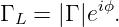
For a lossless line, write the load reflection coefficient as
The voltage is
Its magnitude satisfies
Maximum voltage occurs when the cosine equals +1:
Minimum voltage occurs when the cosine equals −1:
The distance between adjacent maxima is
and the distance from a maximum to the neighboring minimum is
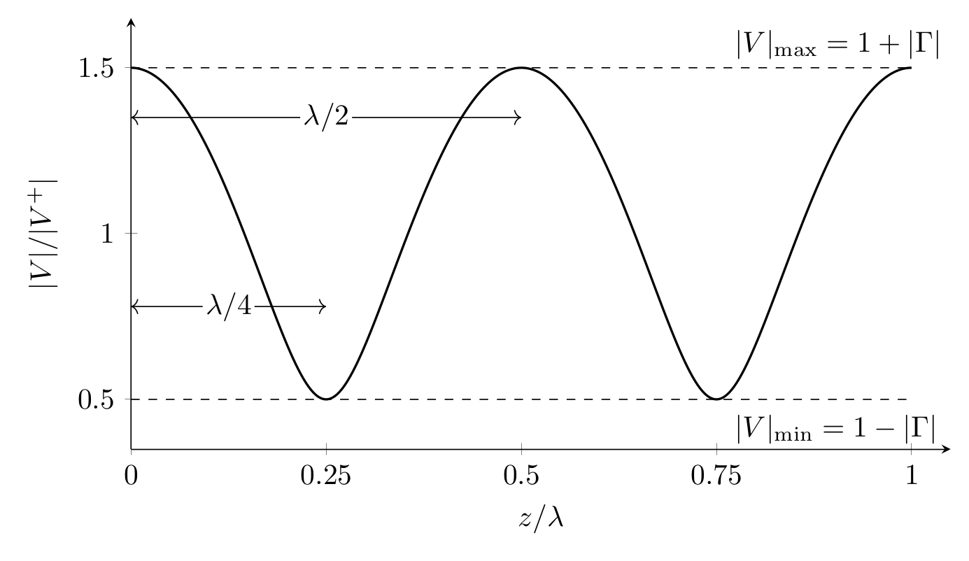
Figure. A reflected wave interferes with the forward wave and produces a spatial
standing-wave envelope. The maximum-to-minimum ratio measures the mismatch
magnitude.
16 Standing-wave ratio
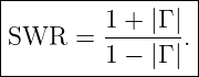
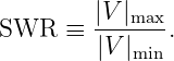
The voltage standing-wave ratio, usually abbreviated VSWR or simply SWR, is
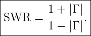
Substituting the extrema gives
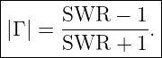
Solving for mismatch magnitude,
Important limiting cases are
| |Γ| = 0 | ⇒ SWR = 1, | (90)
|
| |Γ|→ 1 | ⇒ SWR →∞. | (91) |
SWR measures the magnitude of mismatch but does not determine the phase of Γ.
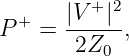
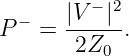
17 Power carried by the forward and reflected waves
For a lossless line with real Z0, the time-average forward power is
and the reflected power magnitude is
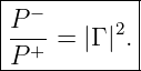
Therefore
The net power flowing toward the load is
This is exactly analogous to EM21, where the reflected power fraction at a lossless material
boundary is R = |Γ|2.
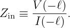
18 Input impedance at an arbitrary distance from the load
A transmission line transforms impedance with distance. For a point a distance ℓ from the load,
located at z = −ℓ, the input impedance is
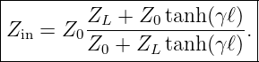
Substituting the forward and reflected solutions and eliminating ΓL gives the general
result
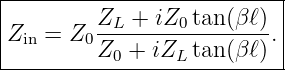
For a lossless line, γ = iβ and
so
This equation explains why a reactive or mismatched load can appear as a very different
impedance when viewed through a finite length of line.
19 Worked example: 50 Ω line terminated in 100 Ω
Consider a lossless line with
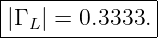
The load reflection coefficient is
| ΓL | =  | (101)
|
| =  . . | (102) |
Thus
The SWR is
| SWR | =  | (104)
|
| = 2. | (105) |
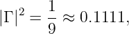
Hence
The reflected power fraction is
so about 11.1% of the incident power is reflected and 88.9% is delivered to the load in this ideal
lossless system.
Now suppose
so
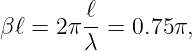
Take a line length
Then
for which
The input impedance is therefore
| Zin | = 50 | (113)
|
| = 40 + i30 Ω. | (114) |
Thus
A purely resistive 100 Ω load has become a complex impedance when viewed through the
line.
20 Quarter-wave and half-wave transformations
Two lossless-line lengths are especially important.
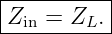
For
we have tan(βℓ) = 0, so
A half-wave line repeats the load impedance.
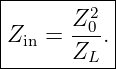
For
| tan(βℓ)|→∞, yielding
This is the quarter-wave impedance inversion. It is the basis of the quarter-wave transformer
developed later in impedance-matching theory.
21 Where L and C come from: a coaxial example
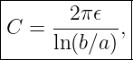
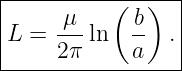
Transmission-line parameters are compact summaries of electromagnetic fields. For an ideal coaxial
line with inner-conductor radius a, outer-conductor inner radius b, permeability μ, and
permittivity 𝜖, electrostatic and magnetostatic field calculations give [3, 5]
and
Therefore
so
This is exactly the bulk electromagnetic-wave speed from EM20.
Likewise,
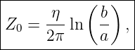
Thus
where
is the intrinsic impedance of the dielectric filling the coax.
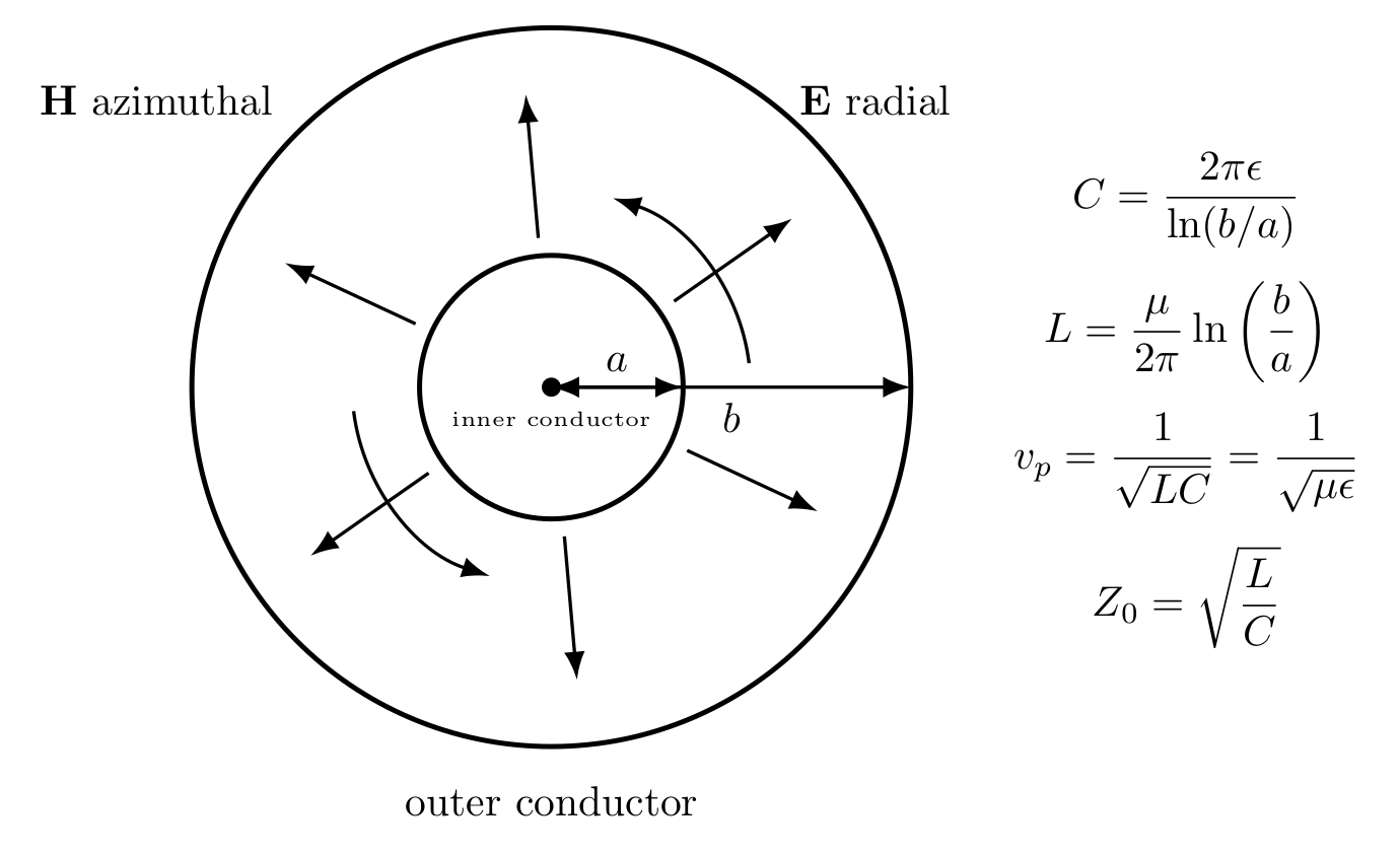
Figure. In a coaxial line, the electric field is primarily radial and the magnetic field is
azimuthal. The distributed C and L encode the same field-energy storage represented
directly by E and H.
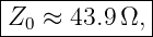
For example, let
Then
so
and
The reduced speed is simply the electromagnetic-wave speed in a dielectric with refractive factor
 = 1.5.
22 Characteristic impedance is not ordinary resistance
The symbol Z0 has units of ohms, but it should not be interpreted as a resistor smeared along the
line. In a lossless line,
yet
remains finite.
The quantity Z0 is the voltage-to-current ratio of a single traveling wave. A matched load equal to
Z0 absorbs the wave energy without reflection; the line itself need not dissipate that
energy.
23 Connection to the electromagnetic boundary problem
The conceptual parallel with EM21 can now be made explicit:
At a material interface,
At a transmission-line load,
In both cases, reflection is created because the forward wave reaches a boundary that demands a
voltage/current or electric/magnetic-field ratio different from that carried by the incident
wave alone. A reflected wave appears so that the total fields can satisfy the boundary
condition.
24 A practical calculation workflow
For a uniform transmission line driven at one frequency:
- identify R,L,G,C and frequency f;
- compute
- compute
- apply the load boundary condition to obtain
- use |Γ| for reflected-power fraction and SWR;
- use the phase of Γ(z) to locate standing-wave maxima and minima;
- if necessary, transform the load through a line length with the input-impedance
equation.
This workflow separates propagation, attenuation, mismatch, and impedance transformation
instead of treating them as unrelated formulas.
25 Common mistakes
- Treating Z0 as a physical resistor. A lossless line can have Z0 = 50 Ω even though
its series resistance is zero.
- Dropping the minus sign in reflected current. The backward wave reverses the
current direction associated with positive power flow.
- Using |Γ| as the reflected power fraction. For a lossless line, the reflected power
fraction is |Γ|2.
- Confusing SWR with reflection phase. SWR determines |Γ|, not the complex
phase of Γ.
- Assuming the load impedance appears unchanged at the source. A finite line
transforms impedance according to its electrical length.
- Using lumped-circuit intuition when the interconnect is electrically long.
Voltage and current become waves with finite propagation speed.
26 What EM22 adds to the series
EM20 established propagation constants and wave impedance in bulk media. EM21 showed how
impedance discontinuities create reflection and standing-wave behavior at material boundaries.
EM22 now translates that physics into the distributed voltage-current language used throughout
RF hardware.
The key results are
and
These equations provide the bridge from electromagnetic wave theory into coaxial cables, PCB
traces, impedance matching, Smith charts, S-parameters, microwave networks, and ultimately the
RF front ends used in communication and navigation receivers.
References
References
[1] D. M. Pozar, Microwave Engineering, 4th ed., Wiley, 2012.
[2] R. E. Collin, Foundations for Microwave Engineering, 2nd ed., Wiley-IEEE Press,
2001.
[3] S. Ramo, J. R. Whinnery, and T. Van Duzer, Fields and Waves in Communication
Electronics, 3rd ed., Wiley, 1994.
[4] F. T. Ulaby and U. Ravaioli, Fundamentals of Applied Electromagnetics, 7th ed.,
Pearson, 2015.
[5] D. K. Cheng, Field and Wave Electromagnetics, 2nd ed., Addison-Wesley, 1989.
[6] C. A. Balanis, Advanced Engineering Electromagnetics, 2nd ed., Wiley, 2012.

















![α [Np/m ]](https://images.physicslibrary.org/cache/objects/1447/make4ht/ElectromagneticWavesAntennasAndRFTransmissionLinesAndTheTelegraphersEquations39x.png)
![β [rad/m ]](https://images.physicslibrary.org/cache/objects/1447/make4ht/ElectromagneticWavesAntennasAndRFTransmissionLinesAndTheTelegraphersEquations40x.png)













![[ ]
V (z) = V +e−iβz 1 + |Γ |ei(2βz+ ϕ) .](https://images.physicslibrary.org/cache/objects/1447/make4ht/ElectromagneticWavesAntennasAndRFTransmissionLinesAndTheTelegraphersEquations80x.png)
![[ ]
|V(z)|2 = |V + |2 1 + |Γ |2 + 2|Γ |cos(2βz + ϕ) .](https://images.physicslibrary.org/cache/objects/1447/make4ht/ElectromagneticWavesAntennasAndRFTransmissionLinesAndTheTelegraphersEquations81x.png)

















 ln
ln