Strapdown Inertial Navigation Examples: Comparing DCM, Euler-Angle, Quaternion, and
Rotation-Vector Propagation
This companion to INS07 uses the same gyroscope data in several attitude representations. The
purpose is not to declare one representation universally superior. The goal is to show that a
direction cosine matrix, Euler Angles, a quaternion, and a rotation vector describe the same
physical orientation when their conventions and numerical propagation are handled
consistently.
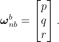
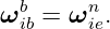
Throughout the article, the gyro rate has already been corrected for navigation-frame
rotation unless a problem explicitly says otherwise. Thus the common propagation input
is
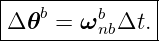
For a short interval Δt over which the rate is approximately constant, define
The DCM update is
the finite quaternion increment is
and
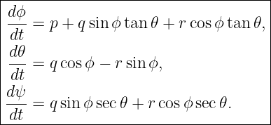
For 3-2-1 roll-pitch-yaw angles,
Finally, a finite rotation vector is
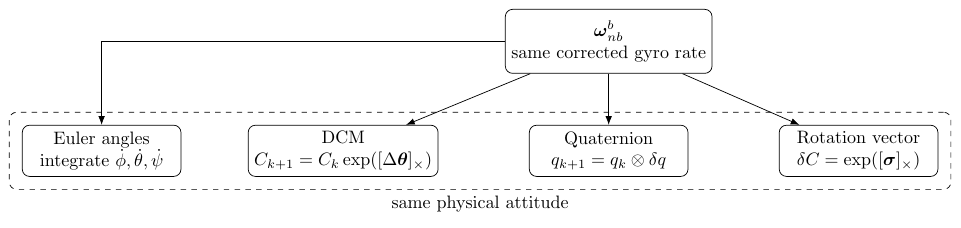
Figure. One corrected gyro-rate vector can drive four attitude representations. The
internal coordinates differ, but a consistent implementation must produce the same
physical orientation.
1 Exercises
Exercise 1: One-axis yaw represented four ways
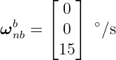
A level vehicle begins aligned with NED and rotates at the constant body-relative rate
for 4 s.
- Compute the final DCM Cbn.
- Compute the final 3-2-1 Euler angles.
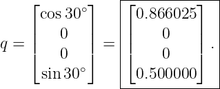
- Compute the scalar-first Hamilton quaternion.
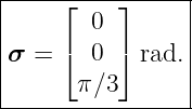
- Compute the finite rotation vector.
- Verify that the quaternion and rotation vector reproduce the DCM.
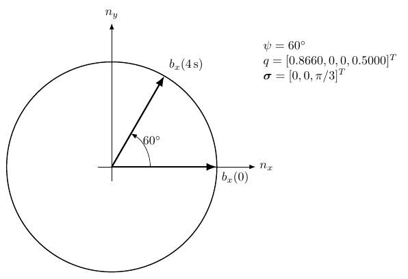
Figure. A pure yaw maneuver is the simplest convention check because all four
representations reduce to a rotation about the same axis.
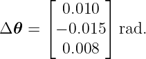
Exercise 2: One finite three-axis gyro increment
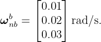
An initially aligned vehicle has
for Δt = 0.25 s.
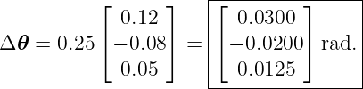
- Form Δ𝜃 and its magnitude α.
- Use Rodrigues’ formula to compute the exact DCM increment.
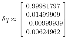
- Compute the equivalent quaternion increment.
- Extract the equivalent 3-2-1 Euler angles from the resulting DCM.
- Show that all representations correspond to the same finite rotation.
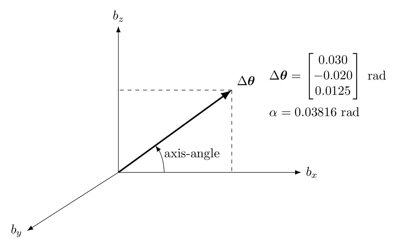
Figure. A three-axis gyro sample defines one finite axis-angle increment. DCM, quaternion,
Euler angles, and rotation vector are different coordinate descriptions of that rotation.
Exercise 3: Euler-angle rate propagation at a nonzero attitude
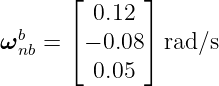
The initial attitude is
and the body-relative rate is
For Δt = 0.02 s:
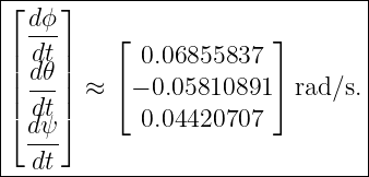
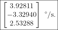
- Compute dϕ∕dt, d𝜃∕dt, and dψ∕dt.
- Use one forward Euler step on the Euler angles.
- Independently propagate the initial DCM using the exact exponential increment.
- Extract Euler angles from that exact DCM and compare the two results.
Exercise 4: Euler-angle singularity with modest gyro rates
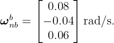
At
suppose
Compute the three Euler-angle rates. Explain why very large roll and yaw rates do not imply a
physically enormous angular velocity. State how DCM, quaternion, and rotation-vector
propagation behave for the same physical rate.
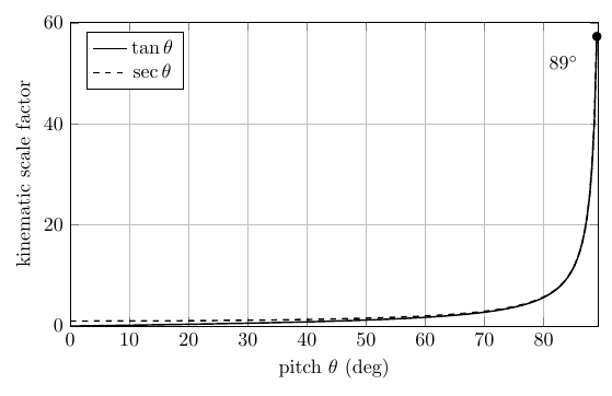
Figure. The 3-2-1 Euler kinematic map contains tan 𝜃 and sec 𝜃. These coordinate scale
factors become large near 90∘ pitch even though the physical angular velocity can remain
small.
Exercise 5: DCM forward Euler versus the exponential map
Reuse the increment from Exercise 2. Beginning from C0 = I, compare
with
Compute CFET C
FE − I, its Frobenius norm, and det CFE. Explain which invariants the exact
update preserves automatically.
Exercise 6: Quaternion forward Euler versus a finite unit quaternion
Again use Exercise 2, beginning from
A first-order step gives
- Compute ∥qFE∥.
- Normalize it.
- Compare the normalized approximation with the exact finite quaternion.
- Compute the attitude-angle difference between the normalized first-order quaternion
and the exact quaternion.
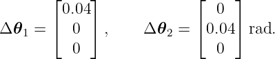
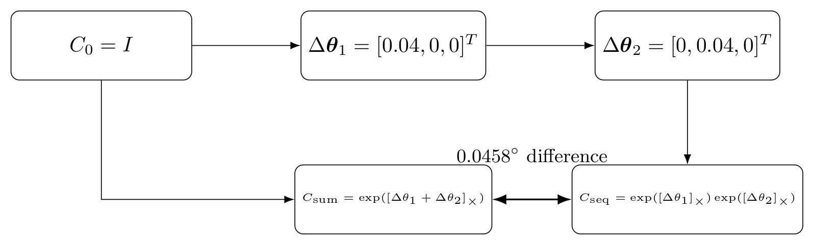
Exercise 7: Two gyro increments that do not commute
Starting from identity attitude, apply
Compare
with the naive single-vector approximation
Find the attitude difference and determine the equivalent rotation vector of the sequential
result.
Exercise 8: A stationary Earth-fixed vehicle
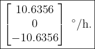
A level vehicle is stationary at latitude 45∘ and aligned with NED. Ignore transport rate. The ideal
gyro therefore measures Earth rate,
- Compute the gyro measurement in rad/s and degrees per hour.
- Compute ωnbb after navigation-frame-rate subtraction.
- State the one-hour attitude change predicted by DCM, Euler-angle, quaternion, and
rotation-vector propagation after the correction.
- Determine the erroneous one-hour rotation magnitude if the raw gyro were integrated
without Earth-rate subtraction.
Exercise 9: Finite increment from a nonidentity attitude
The initial attitude is
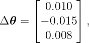
A finite gyro increment is
Propagate the initial attitude once using both DCM multiplication and quaternion multiplication.
Convert both final states to Euler angles and verify agreement.
Exercise 10: Four-sample attitude mechanization comparison
An initially aligned vehicle receives four consecutive corrected gyro samples. Each sample lasts 0.05
s:
| Sample | p (rad/s) | q (rad/s) | r (rad/s) |
|
|
|
|
| 1 | 0.10 | 0.02 | −0.04 |
| 2 | 0.08 | −0.03 | 0.05 |
| 3 | −0.02 | 0.06 | 0.04 |
| 4 | 0.00 | −0.04 | 0.08 |
Propagate the complete sequence using:
- exact DCM increments;
- exact incremental quaternions;
- numerical integration of the 3-2-1 Euler kinematic equations;
- numerical integration of the Bortz rotation-vector equation.
Compare the final attitude from all four methods.
2 Worked solutions
Solution 1: One-axis yaw represented four ways
The angular displacement is
For a positive body z rotation from an initially aligned frame,
The 3-2-1 angles are simply
The unit rotation axis is u = [0, 0, 1]T , so
The rotation vector is
Substitution of the quaternion into the quaternion-to-DCM formula gives the same matrix above.
Rodrigues’ formula with σ does the same. This is a useful unit test for sign, quaternion ordering,
and passive DCM convention.
Solution 2: One finite three-axis gyro increment
The finite increment is
Its magnitude is
Rodrigues’ formula gives
The exact incremental quaternion is
The equivalent Euler angles extracted from δC are
Notice that these Euler angles are not simply the three components of Δ𝜃 converted to degrees.
The rotation-vector components describe one axis-angle rotation, while the Euler angles describe a
sequence of three rotations about different intermediate axes.
Solution 3: Euler-angle rate propagation at a nonzero attitude
With
and
the Euler-rate map gives
In degrees per second,
One forward Euler step over 0.02 s predicts
Now propagate the DCM exactly:
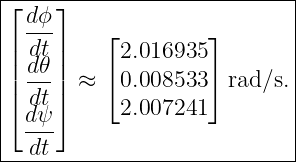
Extracting Euler angles gives
The differences are only about
because the time step is short. The example shows two distinct ideas: the Euler rate
is not the gyro vector, and a numerical Euler-angle integrator still has discretization
error.
Solution 4: Euler-angle singularity with modest gyro rates
At 𝜃 = 89∘,
Substitution gives
In degrees per second,
Yet the physical body rate has magnitude only
The large Euler rates are caused by the coordinate singularity. DCM, quaternion, and
rotation-vector descriptions remain finite for the same physical motion. Their numerical
difficulties are different, but they do not have the 3-2-1 gimbal-lock singularity at this
attitude.
Solution 5: DCM forward Euler versus the exponential map
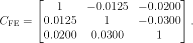
For Exercise 2,
Thus
Its orthogonality defect is
The Frobenius norm is
and
The exact matrix exponential lies on SO(3), so in exact arithmetic
This is one reason finite rotation updates are preferable to repeatedly taking first-order DCM
steps.
Solution 6: Quaternion forward Euler versus a finite unit quaternion
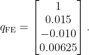
The first-order quaternion is
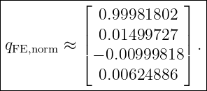
Its norm is
Thus a direct first-order step leaves the unit sphere. After normalization,
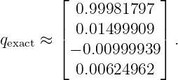
The exact finite quaternion from Exercise 2 is
For two unit quaternions describing nearby attitudes, the relative rotation angle may be obtained
from
Here,
Normalization repairs the quaternion norm, but it does not make a first-order integration step
mathematically identical to the exact finite rotation.
Solution 7: Two gyro increments that do not commute
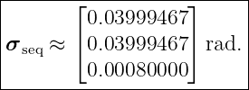
Sequential multiplication gives
The naive sum gives
The relative attitude angle is approximately
The equivalent rotation vector of the sequential result is
The small z component is the key result. It was not present in either individual increment and is
generated by the noncommutative composition. The leading cross term is consistent with the
Baker-Campbell-Hausdorff structure and motivates the coning corrections studied later in the
series [4, 5].
Solution 8: A stationary Earth-fixed vehicle
At 45∘ latitude,
In degrees per hour this is
Because the vehicle is stationary relative to NED,
and therefore
All four correctly driven attitude representations therefore predict zero Earth-relative attitude
change over one hour:
If the raw gyro is integrated as though it were body-relative-to-NED rate, the one-hour rotation
magnitude is
This is a powerful static test for a local-level attitude mechanization.
Solution 9: Finite increment from a nonidentity attitude
Construct the initial DCM from
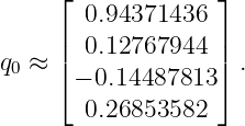
The initial scalar-first quaternion consistent with that DCM is approximately
From
form δC = exp([Δ𝜃]×) and the equivalent δq. Then
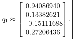
Quaternion propagation gives
Converting either C1 or q1 to Euler angles gives
The maximum elementwise difference between the DCM formed from q1 and the directly
propagated DCM is at floating-point roundoff in this calculation. The order of multiplication is
important. Because the increment is resolved in body coordinates, it multiplies the
body-to-navigation DCM on the right.
Solution 10: Four-sample attitude mechanization comparison
For each sample, form
Sequential exact DCM propagation gives
Sequential finite quaternion propagation gives
The equivalent Euler angles are
Numerically integrating the Euler kinematic equations with a fourth-order method over the same
four piecewise-constant samples gives the same values to the shown precision.
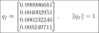
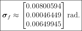
Integrating the Bortz equation gives the final total rotation vector
Applying Rodrigues’ formula to this σf reproduces the DCM above to numerical roundoff.
This exercise is the main lesson of INS07E1. The four state descriptions are not competing physical
models. They are coordinate systems and numerical mechanisms for propagating one underlying
orientation. When the rate convention, frame convention, multiplication order, and numerical
accuracy are consistent, they agree.
3 Cross-method checks for software
The worked examples suggest a compact set of tests for an attitude library.
- One-axis sign test. A positive z rate from identity should produce the expected
positive yaw DCM and quaternion.
- DCM invariant. Verify
- Quaternion invariant. Verify
- Representation agreement. Convert the DCM, quaternion, and rotation vector to one
common DCM and compare matrix elements.
- Euler warning test. Near 𝜃 = ±90∘, do not interpret large Euler rates as large physical
angular velocity.
- Stationary-Earth test. A level Earth-fixed vehicle must have zero NED-relative attitude
rate after Earth-rate subtraction.
- Order test. Swapping two finite cross-axis increments should change the final
attitude.
4 Summary
The DCM, Euler-angle, quaternion, and rotation-vector descriptions all propagate the same
physical attitude, but they expose different numerical properties.
The DCM is geometrically direct and redundant. Exact exponential updates preserve
orthogonality.
Euler angles are intuitive and minimal, but their rate equations depend on the current attitude and
become singular at gimbal lock.
Quaternions are compact and nonsingular for attitude propagation, but they require a unit-norm
constraint and an explicitly stated multiplication convention.
Rotation vectors provide a natural finite-increment description and connect directly
to the exponential map, Rodrigues’ formula, and higher-order strapdown integration
algorithms.
For implementation, the most reliable strategy is to keep one primary nonsingular propagation
state, usually a quaternion or DCM, and derive Euler angles for display. Independent DCM,
quaternion, and rotation-vector implementations are also valuable during development because
agreement among them provides a strong numerical consistency check.
References
[1] David H. Titterton and John L. Weston, Strapdown Inertial Navigation Technology,
2nd ed., Institution of Electrical Engineers, 2004.
[2] Paul D. Groves, Principles of GNSS, Inertial, and Multisensor Integrated Navigation
Systems, 2nd ed., Artech House, 2013.
[3] Christopher Jekeli, Inertial Navigation Systems with Geodetic Applications, Walter
de Gruyter, 2001.
[4] Paul G. Savage, “Strapdown Inertial Navigation Integration Algorithm Design Part
1: Attitude Algorithms,” Journal of Guidance, Control, and Dynamics, vol. 21, no. 1,
pp. 19–28, 1998.
[5] John E. Bortz, “A New Mathematical Formulation for Strapdown Inertial
Navigation,” IEEE Transactions on Aerospace and Electronic Systems, vol. AES-7, no.
1, pp. 61–66, 1971.

![[parent]](https://images.physicslibrary.org/images/uparrow.png)
![Ck+1 = Ck exp ([Δ 𝜃]×),](https://images.physicslibrary.org/cache/objects/1357/make4ht/StrapdownInertialNavigationExamplesComparingDCMEulerAngleQuaternionAndRotationVectorPropagation2x.png)
![[ ] Δ 𝜃
δq = cos(α∕2 ) , α = ∥Δ 𝜃∥, u = ----,
u sin(α∕2) α](https://images.physicslibrary.org/cache/objects/1357/make4ht/StrapdownInertialNavigationExamplesComparingDCMEulerAngleQuaternionAndRotationVectorPropagation3x.png)

![σ = αu, δC = exp([σ ]× ).](https://images.physicslibrary.org/cache/objects/1357/make4ht/StrapdownInertialNavigationExamplesComparingDCMEulerAngleQuaternionAndRotationVectorPropagation6x.png)


![CFE = I + [Δ 𝜃]×](https://images.physicslibrary.org/cache/objects/1357/make4ht/StrapdownInertialNavigationExamplesComparingDCMEulerAngleQuaternionAndRotationVectorPropagation13x.png)
![Cexact = exp([Δ 𝜃]×).](https://images.physicslibrary.org/cache/objects/1357/make4ht/StrapdownInertialNavigationExamplesComparingDCMEulerAngleQuaternionAndRotationVectorPropagation14x.png)
![[ ]
q0 = 1 0 0 0 T .](https://images.physicslibrary.org/cache/objects/1357/make4ht/StrapdownInertialNavigationExamplesComparingDCMEulerAngleQuaternionAndRotationVectorPropagation15x.png)
![[ ]
1
qFE = 1Δ 𝜃 .
2](https://images.physicslibrary.org/cache/objects/1357/make4ht/StrapdownInertialNavigationExamplesComparingDCMEulerAngleQuaternionAndRotationVectorPropagation16x.png)
![Cseq = exp([Δ 𝜃1]×)exp ([Δ 𝜃2]×)](https://images.physicslibrary.org/cache/objects/1357/make4ht/StrapdownInertialNavigationExamplesComparingDCMEulerAngleQuaternionAndRotationVectorPropagation18x.png)
![Csum = exp([Δ𝜃1 + Δ𝜃2 ]× ).](https://images.physicslibrary.org/cache/objects/1357/make4ht/StrapdownInertialNavigationExamplesComparingDCMEulerAngleQuaternionAndRotationVectorPropagation19x.png)










![C1 = C0exp ([ω Δt ]× ).](https://images.physicslibrary.org/cache/objects/1357/make4ht/StrapdownInertialNavigationExamplesComparingDCMEulerAngleQuaternionAndRotationVectorPropagation38x.png)





![⌊ ⌋
0 − 0.0125 − 0.0200
[Δ 𝜃]× = ⌈ 0.0125 0 − 0.0300 ⌉.
0.0200 0.0300 0](https://images.physicslibrary.org/cache/objects/1357/make4ht/StrapdownInertialNavigationExamplesComparingDCMEulerAngleQuaternionAndRotationVectorPropagation45x.png)













![n T
Cb = I, (ϕ,𝜃,ψ ) = (0,0,0), q = [1,0,0, 0] , σ = 0.](https://images.physicslibrary.org/cache/objects/1357/make4ht/StrapdownInertialNavigationExamplesComparingDCMEulerAngleQuaternionAndRotationVectorPropagation65x.png)