Line Integral in Physics: Examples and Complete Worked Solutions
This companion entry develops the ideas from Line Integral in Physics: Curves, work, Circulation,
and Path Dependence through a sequence of worked physics problems. The examples begin with
curve geometry and scalar line integrals, then progress to mechanical work, path dependence,
conservative fields, circulation, Stokes’ theorem, generalized coordinates, and electromagnetic
applications [1, 2, 3, 4].
All exercises are stated first. Complete worked solutions follow afterward so that the first half can
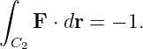
be used as a problem set without revealing the derivations immediately.
Part I: Exercises
Exercise 1: arc length of a straight path
A particle moves along the parameterized curve
Find the arc length of the path using
Exercise 2: a scalar line integral on a quarter circle
Let C be the quarter circle of radius R in the first quadrant,
Evaluate
Then evaluate the result for R = 2 m.
Exercise 3: mass of a nonuniform curved wire
A thin wire forms the same quarter circle of radius R. Its linear mass density is
Find its total mass.
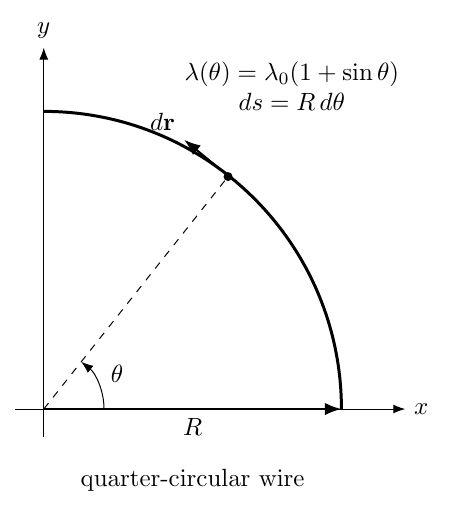
Figure 2. Geometry for Exercise 3. The wire density varies with angular position while ds = Rd𝜃.
Exercise 4: work done by a constant force
A constant force
moves a particle from
to
Find the work. Does the result depend on the path?
Exercise 5: work by a position-dependent force along a straight path
In the plane, let
The particle follows
Evaluate
Exercise 6: work along a curved path
Let
A particle moves along the parabola
Find the work. Then identify a scalar potential Φ such that F = ∇Φ and verify the same answer
from the endpoints.
Exercise 7: path dependence between the same endpoints
Consider
Two paths connect A = (0, 0) to B = (1, 1).
Path C1 goes first from (0, 0) to (1, 0) and then to (1, 1). Path C2 goes first from (0, 0) to (0, 1) and
then to (1, 1).
Evaluate the line integral along each path and show explicitly that the field is path
dependent.
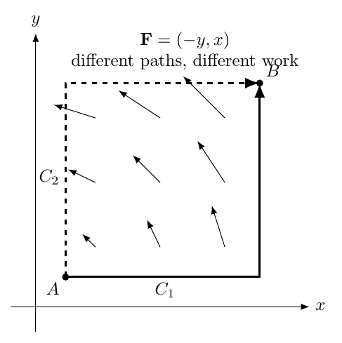
Figure 3. Two piecewise paths for Exercise 7. The vector field produces different work between
the same endpoints.
Exercise 8: conservative field and the potential shortcut
Let
Show that the field is conservative by finding a scalar potential Φ. Then calculate the work
from (0, 0) to (2, 1) without choosing a path. Finally verify the result along the straight
path
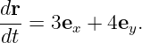
Exercise 9: gravity along a helical path
Near Earth’s surface take
A particle travels along the helix
with 0 ≤ 𝜃 ≤ 2π, where lengths are measured in meters. Find the work done by gravity. Explain
why the radius R does not affect the answer.
Exercise 10: circulation around a circle
For
evaluate the counterclockwise circulation around the circle
Exercise 11: curl-free locally but nonzero circulation
Consider the field
defined away from the origin. Evaluate its counterclockwise line integral around a circle of radius R
centered at the origin. Explain why the result does not contradict the fact that the curl vanishes
away from the origin.
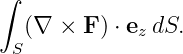
Exercise 12: direct verification of Stokes’ theorem
Let
Let C be the counterclockwise boundary of the disk x2 + y2 ≤ R2 in the xy plane, viewed from +z.
Compute
directly and compare it with
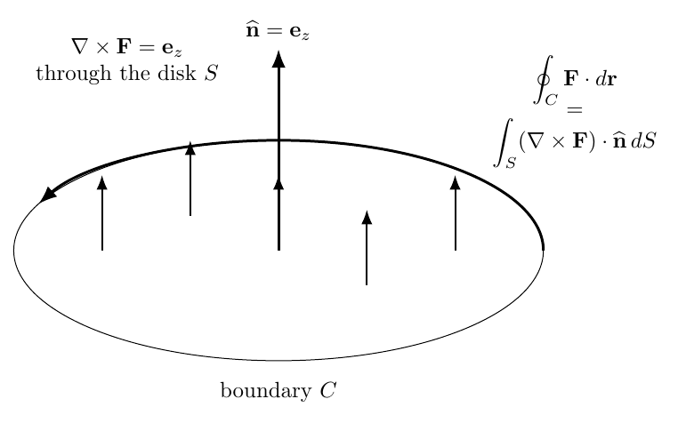
Figure 4. Stokes’ theorem for Exercise 12. Boundary circulation equals the flux of curl through
the spanning disk.
Exercise 13: reparameterization of the same curve
Let
The geometric curve is the parabola y = x2 from (0, 0) to (1, 1).
First use
Then describe the same curve by
Evaluate the line integral in both parameterizations and verify that the results agree.
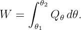
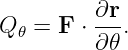
Exercise 14: generalized force for a pendulum
A pendulum bob of mass m and fixed length ℓ has position
Gravity is
Find the generalized force
Then find the work done by gravity as the bob moves from 𝜃1 to 𝜃2. Evaluate the special case
𝜃1 = 0 and 𝜃2 = π∕2.
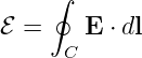
Exercise 15: electromotive-force style circulation
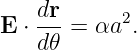
An Electric Field in the plane is
where α is a constant. Find the counterclockwise line integral
around a circle of radius a. Verify the result using Stokes’ theorem.
Exercise 16: synthesis problem on a helical path
A particle moves along
It experiences the force field
Derive the work done over one turn of the helix. Then evaluate the result for
Interpret the two contributions to the work.
Part II: Complete Worked Solutions
Solution 1: arc length of a straight path
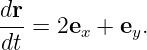
Differentiate the position:
Therefore
The arc-length element is
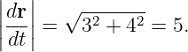
Hence
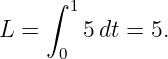
Thus the path length is
The result is simply the length of the straight displacement vector from (0, 0) to (3, 4).
Solution 2: a scalar line integral on a quarter circle
For
we have
Its magnitude is
so
Also
Therefore
Thus
For R = 2 m,
Solution 3: mass of a nonuniform curved wire
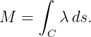
The mass is
For the quarter circle,
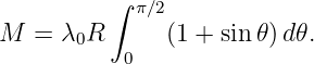
Therefore
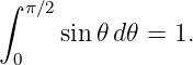
The first part gives π∕2, while
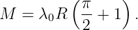
Hence
The result has units of mass because λ0 has units of mass per length and R has units of
length.
Solution 4: work done by a constant force
For a constant force,
The displacement is
Therefore
Thus
Because F is constant, the integral depends only on the net displacement, not on the path taken
between the endpoints.
Solution 5: work by a position-dependent force along a straight path
The path is
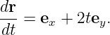
Thus
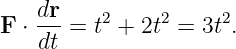
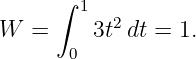
Also
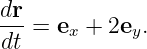
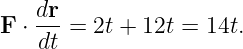
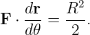
Hence
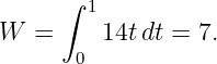
Therefore
So the work is
in the appropriate energy units for the stated force and coordinates.
Solution 6: work along a curved path
Along the parabola,
Therefore
The tangent vector is
Hence
Thus
Now observe that
has gradient
The endpoints are (0, 0) and (1, 1), so
The direct line integral and the potential difference agree.
Solution 7: path dependence between the same endpoints
For C1, the first segment lies along y = 0. There
while dr = dxex, so the dot product is zero.
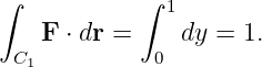
On the second segment, x = 1 and
The field is
Therefore
Hence
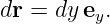
For C2, the first vertical segment has x = 0, so F = −yex and its dot product with dy ey
vanishes.
On the top horizontal segment, y = 1 and
Thus
and
Therefore
The two answers differ:
The field is path dependent. The difference is
which is the counterclockwise circulation around the unit square formed by C1 followed by
−C2.
Solution 8: conservative field and the potential shortcut
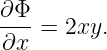
We seek Φ satisfying
Integrating with respect to x gives
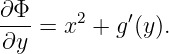
Differentiate with respect to y:
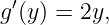
Comparing with the given y component,
Thus
so we may choose
The endpoint method gives
For the straight path x = 2t, y = t,
Also
Therefore
Hence
The explicit path calculation agrees with the potential shortcut.
Solution 9: gravity along a helical path
Only the z component matters because
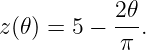
From the path,
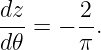
Thus
Therefore
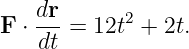
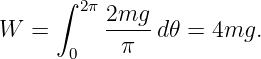
The work is
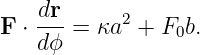
The helix drops from z = 5 m to z = 1 m, a vertical drop of 4 m. Since gravity is conservative,
horizontal motion and the radius R do not change the work.
Solution 10: circulation around a circle
Parameterize the circle by
with 0 ≤ 𝜃 ≤ 2π. Then
Along the circle,
Thus
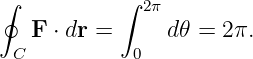
Therefore
Solution 11: curl-free locally but nonzero circulation
On the circle,
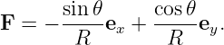
The field becomes
Also
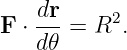
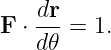
Their dot product is
Hence
The result is independent of R.
The curl vanishes everywhere the field is regular, but the origin is excluded from the domain. A
loop surrounding the origin cannot be continuously contracted to a point without passing through
the singularity. The region is therefore not simply connected, so local curl-free behavior does not
imply global path independence.
Solution 12: direct verification of Stokes’ theorem
On the boundary circle,
The field is
The tangent is
Therefore
Thus
Now calculate the curl. Since
the z component is
Therefore
The surface integral is simply the disk area:
The boundary and surface calculations agree exactly.
Solution 13: reparameterization of the same curve
Using u,
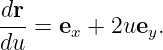
Thus
and
The integrand is
Hence
Using v,
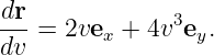
Then
and
Thus the integrand is
Therefore
The two parameterizations describe the same oriented curve, so the geometric line integral is
unchanged.
Solution 14: generalized force for a pendulum
Differentiate the position with respect to 𝜃:
Therefore
Thus
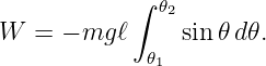
The work is
Hence
Therefore
For 𝜃1 = 0 and 𝜃2 = π∕2,
Gravity does negative work as the bob is raised from its lowest point to the horizontal
position.
Solution 15: electromotive-force style circulation
Parameterize the circle by
Then
and
Thus
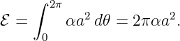
Therefore
For the Stokes check,
Therefore
The two methods agree.
Solution 16: synthesis problem on a helical path
Along the helix,
Therefore the force becomes
The path tangent is
Their dot product is
Using sin 2ϕ + cos 2ϕ = 1,
Hence
Therefore
For the numerical values,
and
Thus
Numerically,
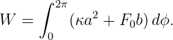
The term 2πκa2 is the work produced by the circulating horizontal field during one revolution. The
term 2πF0b is the work done by the constant axial force through the net vertical displacement
2πb.
References
References
[1] J. R. Taylor, Classical Mechanics, University Science Books, 2005.
[2] J. B. Marion and S. T. Thornton, Classical Dynamics of Particles and Systems, 5th
ed., Brooks/Cole, 2004.
[3] D. J. Griffiths, Introduction to Electrodynamics, 4th ed., Cambridge University Press,
2017.
[4] H. M. Schey, Div, Grad, Curl, and All That: An Informal Text on Vector Calculus,
4th ed., W. W. Norton, 2005.

![[parent]](https://images.physicslibrary.org/images/uparrow.png)




































![2 π∕2 2
I = R [sin 𝜃]0 = R .](https://images.physicslibrary.org/cache/objects/1284/make4ht/ExampleOfLineIntegral46x.png)