Electromagnetic Waves, Antennas, and RF: Maxwell’s Equations as a Complete System
The preceding articles developed the pieces of classical Electromagnetism one at a time: Electric
Charge and Gauss’s Law, current and magnetic fields, Faraday induction, and finally Maxwell’s
displacement-current correction. EM15 now assembles those pieces into a single field
theory.
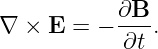
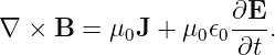
The central objective is not merely to memorize four equations. It is to see how the equations
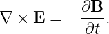
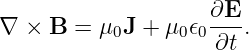
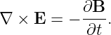
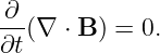
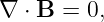
divide into two geometric families:
and
Together they determine how charge density ρ, current density J, electric field E, and magnetic
field B are related in space and time [1, 2, 3, 4, 5].
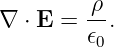
1 The four Maxwell equations in differential form
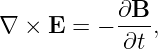
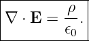
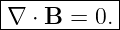
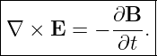
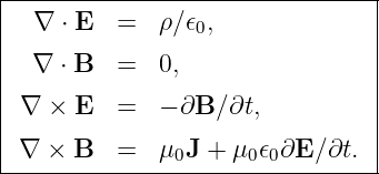
In vacuum with sources ρ and J, Maxwell’s equations are
and
These four equations are local statements. They describe what the fields are doing in an
infinitesimal neighborhood of each point in space and time.
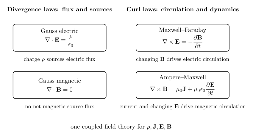
Figure. The four Maxwell equations organized by geometric role. The divergence
equations constrain flux and sources; the curl equations describe circulation and
time-dependent coupling.
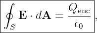
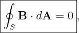
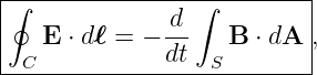
2 The four Maxwell equations in integral form
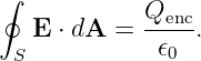
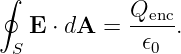
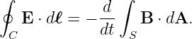
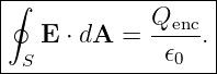
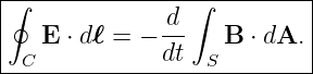
The corresponding integral equations are
and
The first two equations use closed surfaces. The last two use a closed contour C together with a
surface S whose boundary is that contour.
The integral equations are especially useful when symmetry makes flux or circulation simple. The
differential equations are especially useful for local field analysis, partial differential equations, and
wave propagation.
3 Divergence laws: what leaves a small volume?
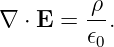
The divergence operator measures local net outward flux per unit volume.
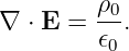
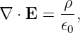
For the electric field,
Positive electric charge acts as a source of outward electric flux; negative charge acts as a
sink.
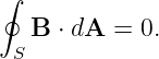
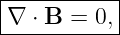
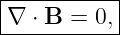
For the magnetic field,
Thus magnetic flux has no local source or sink in classical Maxwell theory. Magnetic field lines do
not begin or end at isolated magnetic charge; their net flux through every closed surface is
zero.
This does not mean that B = 0. A nonzero magnetic field can pass through a closed surface, but as
much flux enters as leaves.
4 Curl laws: what circulates around a small loop?
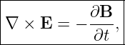
The curl operator measures local circulation.
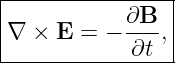
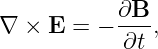
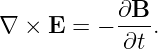
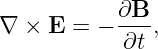
Faraday’s law says
A changing magnetic field therefore produces circulating electric-field structure.
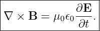
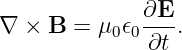
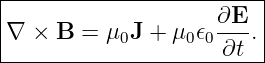
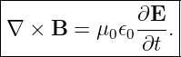
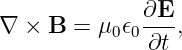
Ampere–Maxwell says
Magnetic circulation can therefore be produced by either conduction current density J or a
changing electric field.
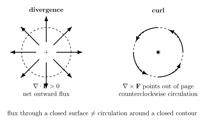
Figure. Divergence and curl answer different geometric questions. Divergence concerns net
flux through a small closed surface; curl concerns circulation around a small loop.
5 Sources versus fields
It is useful to separate the physical quantities into sources and fields.
The source quantities are
The field quantities are
Gauss’s electric law connects ρ directly to the divergence of E. Ampere–Maxwell connects J
directly to part of the curl of B.
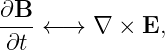
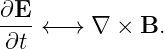
The remaining terms show that the fields are also coupled dynamically to one another:
This is the part of Maxwell’s system that allows electromagnetic disturbances to propagate even
after one moves away from the charges and currents that created them.
6 Integral and differential forms are the same laws at different scales
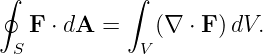
The divergence theorem connects the two versions of the divergence laws:
For Gauss’s electric law,
For Gauss’s magnetic law,
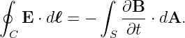
Stokes’ theorem connects the two versions of the curl laws:
Applying this to E gives Faraday’s integral law, while applying it to B gives the Ampere–Maxwell
integral law.
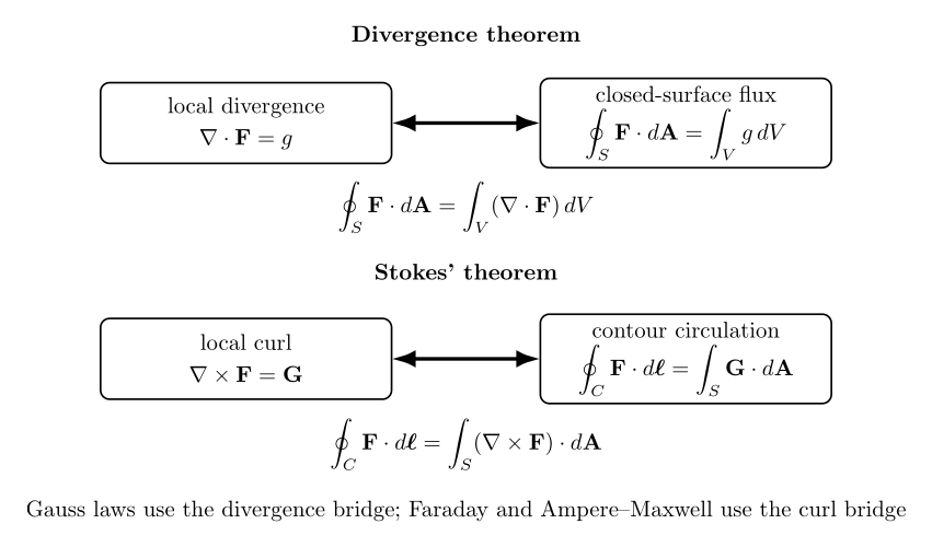
Figure. The divergence theorem bridges closed-surface flux and local divergence. Stokes’
theorem bridges contour circulation and local curl.
7 Example 1: recovering Gauss’s law from the differential equation
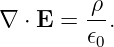
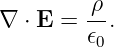
Suppose a region contains uniform charge density ρ0. Gauss’s differential law gives
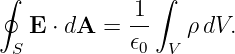
Integrate over a volume V :
Using the divergence theorem,
The integral and differential forms are therefore not separate physical laws; they are equivalent
statements under the usual smoothness assumptions.
8 Example 2: interpreting ∇⋅ B = 0
Suppose magnetic flux enters a closed surface through one region with total inward flux
−4.0 mWb. Gauss’s magnetic law requires
Therefore the remaining portions of the surface must carry total outward flux
The law constrains net flux, not the field magnitude at every point.
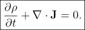
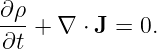
9 Charge conservation is built into the system
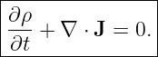
Take the divergence of the Ampere–Maxwell equation:
Since the divergence of a curl vanishes,
where Gauss’s electric law was used.
Hence,
The four Maxwell equations are therefore mutually constrained. Maxwell’s displacement-current
term is precisely what makes the magnetic curl law compatible with time-dependent charge
conservation.
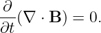
10 Magnetic-flux conservation is also built in
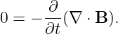
Take the divergence of Faraday’s law:
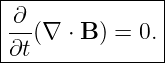
The left side is identically zero, so
Therefore, if
is satisfied initially, Faraday’s law preserves that condition in time.
This is an important structural feature of Maxwell’s system: the divergence constraints and
curl-evolution equations are compatible with one another.
11 Example 3: a local consistency test
Suppose at a point
Gauss’s law gives
Thus,
| ρ | = (8.854 × 10⁻¹²)(2.0 × 10⁴) | (36)
|
| = 1.77 × 10⁻⁷ C/m3. | (37) |
So the local divergence of the electric field directly determines the local charge density.
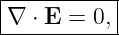
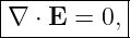
12 The source-free vacuum equations
In a vacuum region containing no charge or conduction current,
Maxwell’s equations reduce to
The divergence equations say that neither field has a local source in that region. The curl
equations say that time variation of each field is tied to circulation of the other.
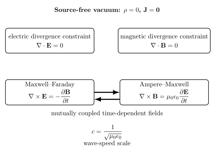
Figure. In source-free vacuum the charge and conduction-current source terms vanish, but
the electric and magnetic fields remain dynamically coupled through the two curl equations.
13 Example 4: the electromagnetic speed scale appears again
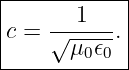
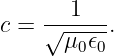
The source-free curl equations contain the product
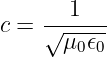
The corresponding speed scale is
Numerically,
The next article will derive the electromagnetic wave equations directly from the source-free
Maxwell system and show why this quantity is the propagation speed.
14 What Maxwell’s equations do not determine by themselves
The differential equations constrain the fields, but solving a physical problem also requires
appropriate information about the domain and boundaries.
Typical additional information includes
- charge and current distributions;
- initial field values;
- Conductor or dielectric boundaries;
- boundary conditions at material interfaces;
- radiation conditions for open-space problems.
Thus Maxwell’s equations are the governing equations, while geometry, sources, and boundary or
initial conditions select the physical solution.
15 A compact interpretation table
The four equations can be remembered structurally:
Gauss electric:
Electric charge sources electric flux.
Gauss magnetic:
There is no net magnetic source flux.
Maxwell–Faraday:
A changing magnetic field drives electric circulation.
Ampere–Maxwell:
Conduction current and a changing electric field drive magnetic circulation.
16 Common mistakes
- Treating the four equations as unrelated formulas rather than one coupled system.
- Confusing divergence with curl: divergence concerns net flux from a point-like
neighborhood, while curl concerns local circulation.
- Interpreting ∇⋅ B = 0 as saying the magnetic field itself must vanish.
- Forgetting the displacement-current term in the Ampere–Maxwell equation.
- Using a closed surface for a curl law or a closed contour for a divergence law without
identifying the associated spanning surface.
- Applying ∇⋅ E = 0 everywhere instead of only in charge-free regions.
- Applying J = 0 everywhere in vacuum-wave problems without first stating that the
chosen region is source-free.
- Treating the integral and differential forms as different physical laws rather than
equivalent formulations connected by the divergence theorem and Stokes’ theorem.
- Forgetting that Maxwell’s equations require boundary and initial conditions to
determine a unique field solution in a particular problem.
Part I: Exercises
All exercises are stated here before any worked solution. Attempt the complete set before
proceeding to Part II.
Exercise 1: identify the Maxwell equation
For each statement below, identify the corresponding Maxwell equation in differential
form.
- Electric charge produces net electric flux.
- Magnetic flux has no local source or sink.
- A changing magnetic field produces electric circulation.
- Conduction current and a changing electric field produce magnetic circulation.
Then classify each equation as a divergence law or a curl law.
Exercise 2: electric divergence and charge density
At some point in vacuum,
Find the local charge density ρ.
Interpret the sign physically.
Exercise 3: magnetic flux through a closed surface
A closed surface is divided into three regions. The signed magnetic fluxes through two regions
are
Use Gauss’s law for magnetism to determine the signed flux through the third region.
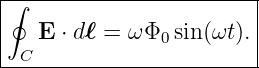
Exercise 4: Faraday circulation from changing magnetic flux
For a fixed contour C, the magnetic flux through a spanning surface is
Find the electric circulation
as a function of time.
State the physical meaning of the minus sign in Faraday’s law.
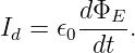
Exercise 5: Ampere–Maxwell circulation with both source terms
A surface bounded by contour C carries enclosed conduction current
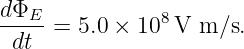
while its electric flux changes at the rate
Find:
- the displacement current;
- the total effective current in the Ampere–Maxwell law;
- the magnetic circulation ∮
CB ⋅ dℓ.
Exercise 6: divergence theorem bridge for Gauss’s law
Starting from
integrate over an arbitrary volume V and use the divergence theorem to derive
Identify the relation between ρ and Qenc used in the derivation.
Exercise 7: Stokes theorem bridge for Faraday’s law
Starting from
integrate over a fixed surface S and use Stokes’ theorem to derive
State why the fixed-surface assumption matters.
Exercise 8: classify a field by divergence and curl
Consider
where a is a constant.
Find:
- ∇⋅ F;
- ∇× F.
Based on those results, explain whether this field is more naturally associated with source-like
behavior, circulation-like behavior, or both.
Exercise 9: a pure rotational field
Consider
where Ω is constant.
Find:
- ∇⋅ F;
- ∇× F.
Explain how this example helps distinguish the geometric meanings of divergence and
curl.
Exercise 10: derive charge continuity from Maxwell’s equations
Starting from the differential Ampere–Maxwell equation,
take the divergence and use Gauss’s electric law to derive
Identify the Vector Identity that makes the derivation possible.
Exercise 11: preservation of the magnetic divergence constraint
Start with Faraday’s law,
Take the divergence of both sides and show that
Explain why this means that if ∇⋅ B = 0 initially, Faraday’s law preserves the condition in
time.
Exercise 12: reduce Maxwell’s equations in source-free vacuum
Begin with the complete differential Maxwell system and impose
Write the resulting four vacuum equations explicitly.
Then identify which two are divergence constraints and which two provide time-dependent field
coupling.
Exercise 13: local consistency test with specified field derivatives
At a point in space and time, suppose
and
Find:
- the local charge density ρ;
- the displacement-current density Jd;
- the total source term J + Jd appearing in the magnetic curl law;
- ∇× B.
Exercise 14: synthesis and bridge to electromagnetic waves
In source-free vacuum, Maxwell’s curl equations are
Answer the following without carrying out the full curl–curl wave-equation derivation:
- explain why a time-varying B field can produce spatial structure in E;
- explain why a time-varying E field can produce spatial structure in B;
- identify the combination of constants that has dimensions of inverse speed squared;
- compute
using
- state why this result strongly suggests that Maxwell’s source-free equations support
waves.
Part II: Complete Worked Solutions
Solution 1: identify the Maxwell equation
For electric charge producing net electric flux,
This is Gauss’s law for electricity, a divergence law.
For magnetic flux having no local source or sink,
This is Gauss’s law for magnetism, also a divergence law.
For a changing magnetic field producing electric circulation,
This is the Maxwell–Faraday law, a curl law.
For conduction current and changing electric field producing magnetic circulation,
This is the Ampere–Maxwell law, also a curl law.
Solution 2: electric divergence and charge density
Gauss’s differential law gives
Thus,
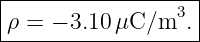
| ρ | = (8.854 × 10⁻¹²)(−3.5 × 10⁵) | (79)
|
| = −3.10 × 10⁻⁶ C/m3. | (80) |
Therefore,
The negative sign means the local electric field has net inward flux behavior, consistent with
negative charge density.
Solution 3: magnetic flux through a closed surface
Gauss’s magnetic law requires
Therefore,
| ΦB3 | = −ΦB1 − ΦB2 | (83)
|
| = −(+2.5) − (−7.0) mWb | (84)
|
| = +4.5 mWb. | (85) |
Hence,
The positive value is the outward flux required to make the total closed-surface magnetic flux
zero.
Solution 4: Faraday circulation from changing magnetic flux
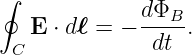
Faraday’s law is
With
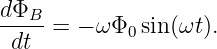
we have
Therefore,
The minus sign in Faraday’s law encodes Lenz’s law: the induced circulation is oriented so that its
electromagnetic response opposes the change in magnetic flux.
Solution 5: Ampere–Maxwell circulation with both source terms
The displacement current is
Thus,
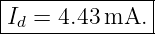
| Id | = (8.854 × 10⁻¹²)(5.0 × 10⁸) | (92)
|
| = 4.43 × 10⁻³ A. | (93) |
Therefore,
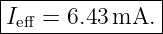
The total effective current is
| Ieff | = Icond,enc + Id | (95)
|
| = 2.00 mA + 4.43 mA | (96)
|
| = 6.43 mA. | (97) |
Hence,
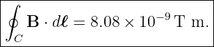
Ampere–Maxwell then gives
| ∮
CB ⋅ dℓ | = μ0Ieff | (99)
|
| = (1.25663706 × 10⁻⁶)(6.43 × 10⁻³) | (100)
|
| = 8.08 × 10⁻⁹ T m. | (101) |
Thus,
The two current-like terms are added because both contribute to the same magnetic circulation
source in the Ampere–Maxwell law.
Solution 6: divergence theorem bridge for Gauss’s law
Begin with
Integrate over an arbitrary volume V :
Apply the divergence theorem to the left side:
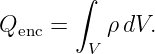
By definition,
Therefore,
Solution 7: Stokes theorem bridge for Faraday’s law
Start with
Integrate over a fixed surface S:
Stokes’ theorem gives
For a fixed surface,
Therefore,
The fixed-surface assumption ensures that the integration domain itself is not moving or changing
shape while the time derivative is taken.
Solution 8: classify a field by divergence and curl
The field is
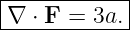
Its divergence is
| ∇⋅ F | =  + +  + +  | (114)
|
| = a + a + a | (115)
|
| = 3a. | (116) |
Thus,
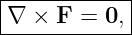
The curl is
because each component depends only on its own coordinate and there are no cross
derivatives.
This field is therefore source-like rather than circulation-like: it has nonzero divergence but zero
curl.
Solution 9: a pure rotational field
The field is
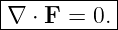
Its divergence is
| ∇⋅ F | =  + +  | (120)
|
| = 0 + 0 | (121)
|
| = 0. | (122) |
Thus,
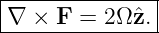
The z component of the curl is
| (∇× F)z | =  − − | (124)
|
| = Ω − (−Ω) | (125)
|
| = 2Ω. | (126) |
The other components vanish, so
This field has circulation without net source-like expansion. It therefore provides a clean geometric
contrast to Exercise 8.
Solution 10: derive charge continuity from Maxwell’s equations
Start from
Take the divergence:
Use
and Gauss’s law
Then
| 0 | = μ0∇⋅ J + μ0𝜖0  | (132)
|
| = μ0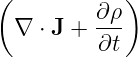 . . | (133) |
Therefore,
The key vector identity is that the divergence of every curl is identically zero.
Solution 11: preservation of the magnetic divergence constraint
Take the divergence of Faraday’s law:
The divergence of a curl is zero, so
Hence,
This means ∇⋅ B is constant in time under Faraday evolution. Therefore, if the initial field
satisfies
it remains zero later.
Solution 12: reduce Maxwell’s equations in source-free vacuum
Set
The four equations become
and
The first two are divergence constraints. The last two are the time-dependent curl equations that
couple the electric and magnetic fields.
Solution 13: local consistency test with specified field derivatives
Gauss’s law gives
Thus,
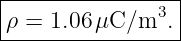
| ρ | = (8.854 × 10⁻¹²)(1.2 × 10⁵) | (145)
|
| = 1.06 × 10⁻⁶ C/m3. | (146) |
Therefore,
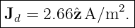
The displacement-current density is
| Jd | = 𝜖0 | (148)
|
| = (8.854 × 10⁻¹²)(3.0 × 10¹¹)z | (149)
|
| = 2.656z A/m2. | (150) |
Hence,
The total current-like source is
| J + Jd | = (0.40 + 2.656)z | (152)
|
| = 3.056z A/m2. | (153) |
Thus,
Ampere–Maxwell gives
| ∇× B | = μ0(J + Jd) | (155)
|
| = (1.25663706 × 10⁻⁶)(3.056)z | (156)
|
| = 3.84 × 10⁻⁶z T/m. | (157) |
Therefore,
Solution 14: synthesis and bridge to electromagnetic waves
Faraday’s law,
states that a changing magnetic field is accompanied by electric-field circulation. Thus time
dependence in B creates spatial structure in E.
Ampere–Maxwell in source-free vacuum,
states that a changing electric field is accompanied by magnetic-field circulation. Thus time
dependence in E creates spatial structure in B.
The constant combination
has dimensions of inverse speed squared. Therefore define
Substituting the given constants gives
| c | =  | (163)
|
| ≈ 2.998 × 10⁸ m/s. | (164) |
Hence,
Because each time-varying field is tied to spatial circulation of the other, the source-free system
contains the feedback structure needed for propagation. The appearance of a definite speed
constructed from μ0 and 𝜖0 strongly signals a wave equation. The next article will carry out that
derivation explicitly.
17 What EM15 adds to the series
EM14 completed the time-dependent magnetic curl law. EM15 places all four equations into one
coherent mathematical structure:
The two divergence equations constrain source and flux structure. The two curl equations govern
circulation and time-dependent field coupling. The next step is to combine the vacuum
curl equations with vector identities and derive the electromagnetic wave equations
directly.
References
[1] David J. Griffiths, Introduction to Electrodynamics, 4th ed., Cambridge University
Press, 2017.
[2] Edward M. Purcell and David J. Morin, Electricity and Magnetism, 3rd ed.,
Cambridge University Press, 2013.
[3] Samuel J. Ling, Jeff Sanny, and William Moebs, University Physics, Volume 2,
OpenStax, 2016, sections on Maxwell’s equations and electromagnetic waves.
[4] Richard P. Feynman, Robert B. Leighton, and Matthew Sands, The Feynman Lectures
on Physics, Volume II, Addison-Wesley, 1964, chapters on Maxwell’s equations and
electromagnetic radiation.
[5] Massachusetts Institute of Technology, 8.02 Physics II: Electricity and Magnetism,
MIT OpenCourseWare, materials on Maxwell’s equations, Gauss’s law, Faraday
induction, Ampere–Maxwell law, and electromagnetic waves.