Electromagnetic Waves, Antennas, and RF: The Laplacian and the 3D Wave Equation

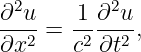
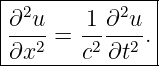
The wave mechanics series developed the one-dimensional wave equation

|-2---------2--| |∂-u-= 1-∂-u-.| -∂x2----c2∂t2---

(1)

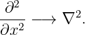
That equation describes a field that varies along one spatial coordinate. Radio waves, however, propagate through three-dimensional space. The purpose of EM04 is to replace the one-dimensional curvature operator

2 -∂-- ∂x2

(2)

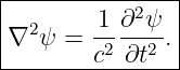
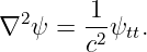
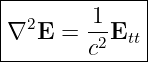
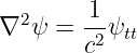
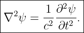
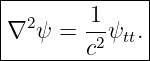
with its three-dimensional counterpart, the Laplacian, and thereby obtain the three-dimensional wave equation

|-----------2--| | 2 1-∂-ψ- | ∇--ψ-=--c2-∂t2 .

(3)

The article remains deliberately mathematical. Maxwell’s equations have not yet been introduced. Later in the series, Maxwell’s equations will show why electric and magnetic fields satisfy this same wave-equation structure in source-free homogeneous regions [2, 5].

1 Why a second spatial derivative appeared in the 1D wave equation

For a one-dimensional field u(x,t), the first derivative

∂u- ∂x

(4)

measures local slope. The second derivative

∂2u --2- ∂x

(5)

measures how that slope changes from point to point. Geometrically, it measures local curvature along the x direction.

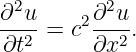
For a stretched string, this curvature enters the net transverse force and therefore the transverse acceleration. The result derived in the Wave Mechanics series is

∂2u- 2∂2u- ∂t2 = c ∂x2 .

(6)

Written with the spatial term first,

|-------1----| |uxx = --utt.| -------c2----|

(7)

The important structural lesson is that spatial curvature is tied to temporal acceleration.

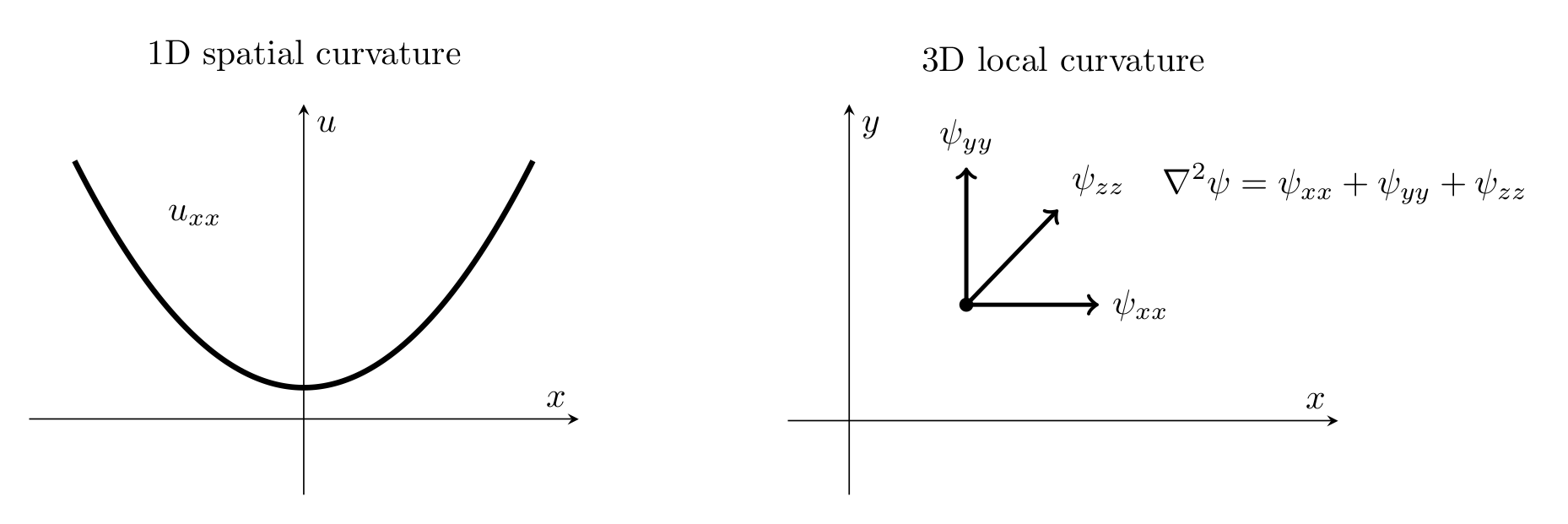
Figure. The one-dimensional second derivative measures curvature along one spatial axis. In three dimensions the Laplacian adds the second-derivative contributions from the three Cartesian directions.

2 Second derivatives in three spatial dimensions

Consider a scalar field

ψ = ψ (x,y,z,t).

(8)

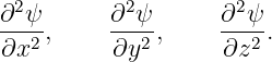
At a fixed time, the field can curve independently along x, y, and z. The three Cartesian second derivatives are

∂2ψ ∂2 ψ ∂2ψ --2-, ---2 , ---2 . ∂x ∂y ∂z

(9)

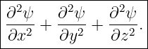
The simplest rotationally symmetric way to combine these Cartesian curvature contributions is to add them:

|-------------------| ∂2 ψ ∂2 ψ ∂2 ψ | ---2 + ---2 + ---2 .| -∂x-----∂y-----∂z----

(10)

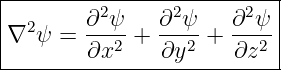
This combination is the Cartesian Laplacian.

3 The Laplacian

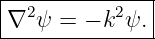
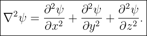
The Laplacian of a scalar field is written

|----| ∇2-ψ--

(11)

and in Cartesian coordinates is defined by

|--------------------------| | 2 ∂2ψ- ∂2ψ- ∂2ψ- | |∇ ψ = ∂x2 + ∂y2 + ∂z2 .| ----------------------------

(12)

The notation ∇² is read “del squared” or “the Laplacian.”

3.1 The Laplacian is divergence of the gradient

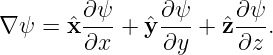
EM03 introduced

∂-ψ ∂ψ- ∂ψ- ∇ ψ = ˆx ∂x + ˆy ∂y + ˆz∂z .

(13)

Take the divergence of this vector field:

∇⋅ (∇ψ)	= + +	(14)
	= + + .	(15)

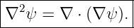
Therefore,

|-----------------| ∇2 ψ = ∇ ⋅ (∇ ψ).| -------------------

(16)

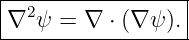
This identity gives the Laplacian a useful interpretation: first form the field pointing toward fastest increase, then ask whether that gradient field has local net outward flux.

Figure. The Laplacian maps a scalar field to another scalar field by taking the divergence of its gradient.

3.2 Operator type

The gradient maps

scalar − → vector,

(17)

while divergence maps

vector −→ scalar.

(18)

Therefore the Laplacian maps

|-----------------| scalar − → scalar. | -------------------

(19)

This type check is useful whenever a long expression involving ∇ becomes difficult to read.

3.3 Units

If ψ has units [ψ], then every spatial derivative contributes one inverse length. Therefore

|------------| [∇2 ψ] = [ψ].| ---------m2---

(20)

This will match the right-hand side of the wave equation because

[ ] -1 ∂2ψ- -s2[ψ-] [ψ-] c2 ∂t2 = m2 s2 = m2 .

(21)

4 A geometric interpretation of the Laplacian

In one dimension, a positive second derivative means the curve is locally concave upward. A negative second derivative means it is locally concave downward.

The Laplacian generalizes this idea by adding the local curvature contributions from independent spatial directions. Roughly speaking:

∇²ψ	> 0	means the field is locally bowl-like,	(22)
∇²ψ	< 0	means the field is locally cap-like,	(23)
∇²ψ	= 0	means positive and negative curvature contributions balance locally.	(24)

This interpretation is local. The Laplacian is not the field value itself, and a field can be nonzero while its Laplacian is zero.

5 Worked example 1: Laplacian of a polynomial field

Let

2 2 2 ψ (x,y,z) = x + 2y − 3z + 4xy.

(25)

The second derivatives are

2 2 2 ∂-ψ-= 2, ∂--ψ = 4, ∂-ψ- = − 6. ∂x2 ∂y2 ∂z2

(26)

Therefore,

∇²ψ	= 2 + 4 − 6	(27)
	= 0.	(28)

Hence

|----------| |∇2 ψ = 0. | -----------

(29)

Notice that the mixed term 4xy contributes no second derivative to the Cartesian Laplacian because

∂2(4xy) ∂2(4xy ) ----2---= 0, -----2-- = 0. ∂x ∂y

(30)

6 Harmonic fields

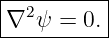
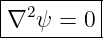
A scalar field satisfying

|--------| ∇2 ψ = 0| ----------

(31)

is called a harmonic field, and the equation itself is Laplace’s equation.

This equation appears throughout electrostatics, gravitation, steady heat flow, and potential theory. It is not yet a wave equation because it contains no time derivative.

The distinction is important:

|-------------------------------| | 2 | Laplace-equation:-----∇--ψ-=-0,--

(32)

whereas

|--------------------------------| | 2 -1 | -wave-equation:-----∇-ψ--=-c2ψtt.-

(33)

7 From the 1D wave equation to the 3D wave equation

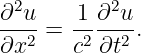
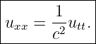
The one-dimensional equation is

∂2u- 1-∂2u- ∂x2 = c2∂t2 .

(34)

If a field may vary independently in all three spatial directions, replace the one-dimensional spatial curvature by the Laplacian:

∂2 ----−→ ∇2. ∂x2

(35)

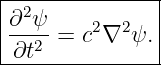
This gives

|--------------| | 2 1 ∂2ψ | ∇ ψ = -2---2 .| --------c--∂t---

(36)

Equivalently,

|--------------| |∂2ψ 2 2 | |--2-= c ∇ ψ. | -∂t-------------

(37)

This is the scalar three-dimensional wave equation in a homogeneous isotropic medium with constant wave speed c [3, 6].

7.1 What the equation says physically

The equation equates two local quantities:

temporal acceleration ← → spatial curvature.

(38)

If the field bends spatially, the wave equation dictates how the field must accelerate in time. Conversely, rapid temporal acceleration requires corresponding spatial curvature.

8 The 1D equation is contained inside the 3D equation

Suppose

ψ (x,y,z,t) = u(x, t),

(39)

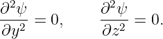
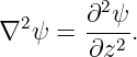
so the field does not depend on y or z. Then

∂2 ψ ∂2ψ ---2 = 0, ---2 = 0. ∂y ∂z

(40)

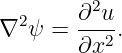
Therefore,

2 ∇2ψ = ∂-u-. ∂x2

(41)

The 3D wave equation becomes

∂2u- 1-∂2u- ∂x2 = c2∂t2 ,

(42)

which is exactly the familiar one-dimensional result.

9 Worked example 2: reduce a 3D equation to 1D

Let

ψ (x,y,z,t) = A cos(kz − ωt).

(43)

Because the field depends on z but not on x or y,

2 ∂2ψ- ∇ ψ = ∂z2 .

(44)

Thus even though the field exists in three-dimensional space, its spatial dependence is effectively one-dimensional.

This distinction is important. A three-dimensional field need not vary in all three coordinates.

10 Plane waves in three dimensions

EM02 introduced the three-dimensional plane-wave phase

𝜃(r,t) = k ⋅ r − ωt.

(45)

A scalar plane wave can therefore be written

|-------------------------------| ψ-(r,t) =-A-cos(k-⋅ r-−-ωt-+-ϕ0).

(46)

Here

k = kxˆx + kyˆy + kz ˆz

(47)

is the wave vector, and

|-------| k-=-|k|--

(48)

is the scalar Wavenumber.

The constant-phase surfaces satisfy

k ⋅ r = C

(49)

at fixed time, so they are planes normal to k.

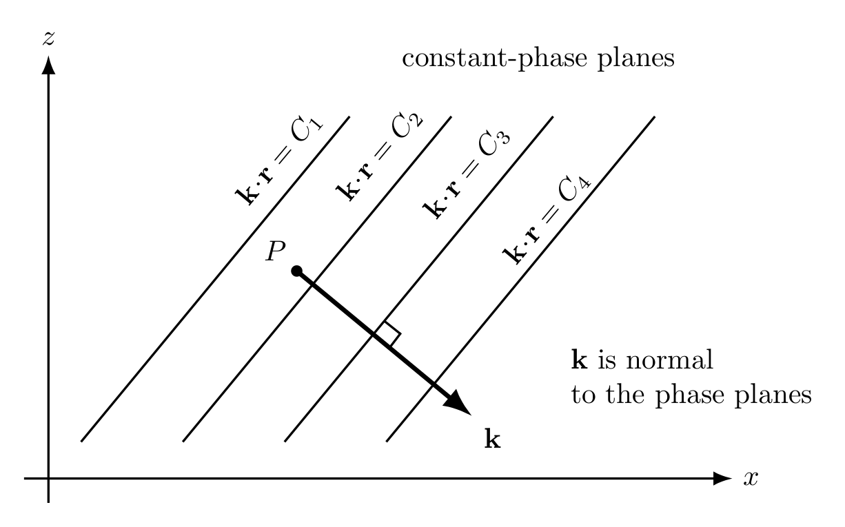
Figure. A plane wave has parallel constant-phase planes. The wave vector k is normal to those planes and points in the propagation direction.

11 Verify that a plane wave satisfies the 3D wave equation

Let

ψ (r,t) = A cos𝜃,

(50)

where

𝜃 = k ⋅ r − ωt + ϕ0.

(51)

Write

k ⋅ r = kxx + kyy + kzz.

(52)

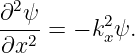
Differentiating twice with respect to x gives

∂2ψ ---- = − k2xψ. ∂x2

(53)

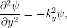
Similarly,

∂2ψ ---- = − k2yψ, ∂y2

(54)

and

∂2ψ- 2 ∂z2 = − kzψ.

(55)

Therefore,

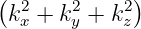∇²ψ	= −ψ	(56)
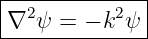
	= −k²ψ.	(57)

Thus

|--2-------2---| -∇--ψ-=-−-k-ψ.-|

(58)

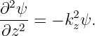
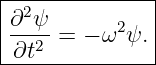
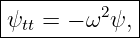
Now differentiate twice with respect to time:

|--------------| |∂2ψ 2 | |---2 = − ω ψ. | -∂t------------

(59)

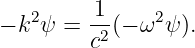
Substitute these into the 3D wave equation:

− k2ψ = 1-(− ω2ψ ). c2

(60)

For a nonzero wave field,

2 ω2- k = c2 .

(61)

Taking the positive-frequency branch,

|--------| -ω-=-ck.-|

(62)

This is the nondispersive dispersion relation for the ideal constant-speed wave equation.

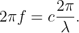
12 Frequency, wavelength, and wave speed

Recall

ω = 2πf

(63)

and

2π- k = λ .

(64)

Substituting into

ω = ck

(65)

gives

2π- 2πf = c λ .

(66)

Hence

|--------| |c = fλ. | ---------

(67)

The familiar one-dimensional relation therefore survives unchanged in three dimensions. The new information carried by k is the propagation direction.

13 Worked example 3: wave vector, wavelength, and direction

Suppose

ˆ ˆ k = 3 x + 4zrad/m.

(68)

The scalar wavenumber is

√ ------- k = 32 + 42 = 5 rad/m.

(69)

Therefore,

2π- 2π- λ = k = 5 m ≈ 1.257m.

(70)

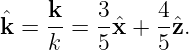
The propagation unit vector is

ˆ k- 3- 4- k = k = 5ˆx + 5ˆz.

(71)

Thus

|----------------------------------| -λ-≈-1.257-m,-----ˆk-=--0.6xˆ+--0.8ˆz.-|

(72)

14 Worked example 4: determine frequency from a 3D wave vector

Suppose a wave travels with

c = 3.00 × 108 m/s

(73)

and has

|k | = 32.96 rad/m.

(74)

Then

ω = ck = (3.00 × 108)(32.96 ) ≈ 9.888 × 109 rad/s.

(75)

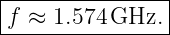
The frequency is

f	=	(76)
	≈ 1.574 × 10⁹ Hz.	(77)

Thus

|---------------| f ≈ 1.574 GHz. | -----------------

(78)

This is close to the GPS L1 carrier frequency. The point here is not yet GPS link analysis, but the direct connection among wave vector, wavelength, and radio frequency.

15 Any waveform can travel along a fixed direction

A sinusoid is not the only possible solution. Let

s = ˆn ⋅ r − ct,

(79)

where n is a constant unit vector. Consider

ψ (r,t) = F(s).

(80)

Using the chain rule,

∇ ψ = F ′(s)nˆ.

(81)

Taking the divergence,

∇2 ψ = F ′′(s)(nˆ⋅ ˆn).

(82)

Because n is a unit vector,

ˆn ⋅ ˆn = 1,

(83)

2 ′′ ∇ ψ = F (s).

(84)

The time derivatives give

∂2ψ ---2 = c2F ′′(s). ∂t

(85)

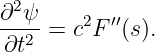
Hence

∇2 ψ = 1-ψtt. c2

(86)

Therefore,

|----------------------| |ψ(r,t) = F (ˆn ⋅ r − ct)| -----------------------

(87)

is a traveling-wave solution for any sufficiently smooth waveform F.

This is the three-dimensional counterpart of the one-dimensional traveling form F(x − ct).

16 Spherical waves: a preview of radiation spreading

Plane waves are useful locally and mathematically, but a compact source radiating into open three-dimensional space does not produce infinite planar wavefronts. Far from an ideal point-like source, the wavefronts are approximately spherical.

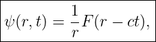
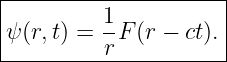
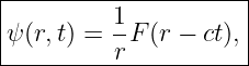
Away from the source point, for r > 0, a common outgoing spherical-wave form is

|---------1----------| ψ (r,t) = -F (r − ct),| ----------r-----------

(88)

where

∘ ------------ r = x2 + y2 + z2.

(89)

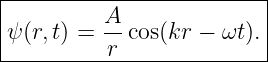
For a sinusoid,

|------------------------| | A- | ψ (r,t) = r cos(kr − ωt).| --------------------------

(90)

The important new feature is the factor

1 -. r

(91)

The field amplitude decreases approximately as 1∕r because the wave spreads across larger spherical surfaces as it propagates outward.

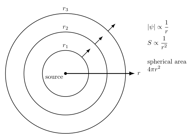
Figure. An outgoing spherical wave spreads over surfaces whose area grows as 4πr². Field amplitude scales approximately as 1∕r in the radiation region, while power flux later scales as 1∕r².

16.1 Why this matters for radio

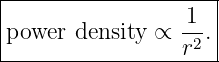
If field amplitude scales as

1- |ψ | ∝ r,

(92)

and wave power density is proportional to field amplitude squared, then

|--------------------| |power density ∝ 1-.| ------------------r2-|

(93)

Later articles will derive this carefully using electromagnetic energy flux and the Poynting vector. This is the mathematical seed of free-space spreading loss and, eventually, the Friis transmission equation.

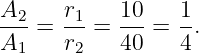
17 Worked example 5: spherical-wave amplitude ratio

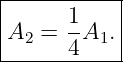
Suppose the far-field amplitude at r₁ = 10 m is A₁. At r₂ = 40 m,

A2 r1 10 1 --- = -- = ---= --. A1 r2 40 4

(94)

Thus

|-----1----| A2 = --A1.| ------4-----

(95)

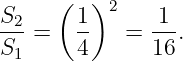
If power density is proportional to amplitude squared, then

( ) S2- 1- 2 -1- S = 4 = 16 . 1

(96)

This anticipates the inverse-square behavior that will become central to RF link budgets.

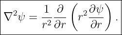
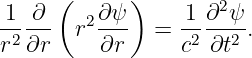
18 The radial Laplacian

The Cartesian definition of the Laplacian is fundamental, but spherical symmetry is easier to describe using the radius r. If a scalar field depends only on r and t, then for r > 0 the Laplacian reduces to

|------------(------)---| | 2 1--∂- 2∂ψ- | ∇ ψ = r2∂r r ∂r . | ------------------------

(97)

This formula will be derived more fully when spherical waves and radiation geometry are developed in later articles. For now, it explains why the factor 1∕r naturally appears in outgoing three-dimensional waves.

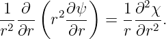
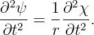
19 Worked example 6: the radial wave equation simplifies after multiplying by r

For spherical symmetry, the wave equation is

( ) 2 1--∂- r2∂ψ- = 1-∂-ψ-. r2∂r ∂r c2 ∂t2

(98)

Define

χ (r,t) = rψ (r,t).

(99)

Then

χ ψ = r-.

(100)

A direct differentiation gives

( ) 1--∂- 2∂-ψ 1-∂2χ- r2∂r r ∂r = r ∂r2 .

(101)

Also,

∂2ψ 1 ∂2χ ---2 = ----2-. ∂t r ∂t

(102)

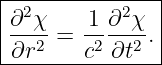
Therefore the radial wave equation becomes

|--------------| |∂2χ 1 ∂2χ | |--2-= -2---2 . -∂r-----c-∂t----

(103)

So χ = rψ obeys an ordinary one-dimensional wave equation in the radial coordinate. An outgoing solution is

χ = F (r − ct),

(104)

which gives

|---------1----------| ψ (r,t) = -F (r − ct).| ----------r-----------

(105)

This is the mathematical origin of the 1∕r spherical spreading factor.

20 Vector fields and the vector wave equation

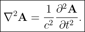
Electromagnetism uses vector fields such as E and B. In Cartesian coordinates, the Laplacian of a vector field can be applied component by component:

|----------------------------------------| |∇2A = (∇2Ax )ˆx + (∇2Ay )ˆy + (∇2Az )ˆz.| -----------------------------------------

(106)

A vector wave equation therefore has the form

|----------------| | 2 1-∂2A-- | |∇ A = c2 ∂t2 .| -----------------

(107)

In a fixed Cartesian basis, this represents three scalar wave equations, one for each field component.

Later, Maxwell’s equations will lead to wave equations of this form for the electric and magnetic fields in source-free homogeneous media.

21 Worked example 7: a polarized vector plane wave

Consider

E (z,t) = E0 cos(kz − ωt)ˆx.

(108)

The only nonzero component is

Ex = E0 cos(kz − ωt).

(109)

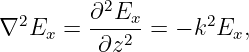
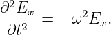
Its Laplacian is

2 ∂2Ex- 2 ∇ Ex = ∂z2 = − k Ex,

(110)

while

∂2Ex ---2- = − ω2Ex. ∂t

(111)

Therefore this component satisfies the wave equation when

ω = ck.

(112)

Because the basis vector x is constant,

|-------------| ∇2E = 1-E | --------c2--tt--

(113)

under the same condition.

This is an early mathematical model of a linearly polarized plane wave. The physical reason that electromagnetic fields satisfy such an equation will come later from Maxwell’s equations.

22 Common mistakes

22.1 Treating ∇² as the square of an ordinary number

The notation

∇2

(114)

means a second-order differential operator. It is not ordinary multiplication of a numerical quantity ∇ by itself.

22.2 Forgetting that k and k are different objects

The vector

k

(115)

contains both direction and magnitude. The scalar

k = |k|

(116)

is the wavenumber appearing in

2π- k = λ .

(117)

22.3 Assuming a 3D field must depend on all three coordinates

A field such as

ψ (z,t)

(118)

can exist throughout three-dimensional space while varying only along z. The unused derivatives simply vanish.

22.4 Confusing the Laplace equation with the wave equation

The equations

2 ∇ ψ = 0

(119)

and

1 ∇2 ψ = -2ψtt c

(120)

have different physical content. The first is time independent; the second describes propagation.

22.5 Forgetting the 1∕r amplitude factor for spherical waves

A sinusoidal phase

cos(kr − ωt)

(121)

by itself does not describe the usual outgoing spherical solution in three dimensions. The radiation-region solution includes the geometric spreading factor

1- r.

(122)

23 Summary

The central results of EM04 are:

|--------------------------| | 2 ∂2-ψ ∂2-ψ ∂2-ψ | |∇ ψ = ∂x2 + ∂y2 + ∂z2 | ---------------------------

(123)

and

|-2---------------| ∇--ψ-=--∇-⋅ (∇-ψ).-

(124)

The scalar three-dimensional wave equation is

|--------------| | 2 1- | |∇ ψ = c2ψtt.| ---------------

(125)

For a plane wave,

ψ = A cos(k ⋅ r − ωt + ϕ0),

(126)

we found

--------------- | 2 2 | ∇--ψ-=--− k-ψ--

(127)

and

|---------2--| -ψtt =-−-ω-ψ,-

(128)

which require

|--------| -ω-=-ck.-|

(129)

For a spherically spreading outgoing wave,

|---------1----------| ψ (r,t) = -F (r − ct),| ----------r-----------

(130)

so field amplitude falls as 1∕r before any electromagnetic power calculation is introduced.

EM05 next moves from this mathematical field language to the first electromagnetic field itself: Electric Charge and the Electric Field.

References

[1] H. M. Schey, Div, Grad, Curl, and All That, 4th ed., W. W. Norton & Company, 2005.

[2] David J. Griffiths, Introduction to Electrodynamics, 4th ed., Cambridge University Press, 2017.

[3] Walter A. Strauss, Partial Differential Equations: An Introduction, 2nd ed., Wiley, 2007.

[4] Gilbert Strang and Edwin “Jed” Herman, Calculus, Volume 3, OpenStax, 2016, chapters on vector calculus and second-order differential operators.

[5] Samuel J. Ling, Jeff Sanny, and William Moebs, University Physics, Volume 2, OpenStax, 2016, chapters on electromagnetic waves.

[6] Frank S. Crawford, Jr., Waves, Berkeley Physics Course, Volume 3, McGraw-Hill, 1968.

[7] Massachusetts Institute of Technology, 8.03SC Physics III: Vibrations and Waves, MIT OpenCourseWare, materials on wave equations and traveling waves.

"Antennas Electromagnetic Waves" is owned by bloftin.
(view preamble)