
|
|
|
|||||||
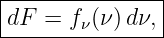
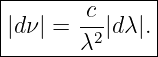
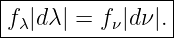
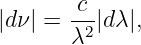
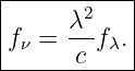
Using
we obtain
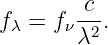
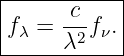
Hence
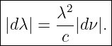
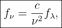
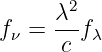
Solving for fν gives
Since
the same relations can be written
provided the two functions are evaluated at corresponding frequency and wavelength.
8 The numerical value depends on the spectral coordinateThe quantities
and
describe the same physical radiation, but their numerical values are generally very different. This is because they are densities with respect to different coordinates. A useful analogy is population density:
and
The underlying population is the same, but the numerical density changes because the unit interval changes. For spectra, the coordinate transformation is not merely a constant unit conversion. The factor
changes with wavelength.
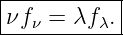
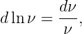
9 A useful invariant per logarithmic intervalMultiply the conversion relation
by
Then
This quantity represents flux per logarithmic spectral interval. Indeed,
so
Likewise,
in magnitude. Plots of
or
are therefore especially useful for comparing energy contributions across logarithmic portions of a broad spectrum.
10 The same spectrum can look different in
|
 | (58) |
Then
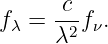 | (59) |
Therefore the same source has
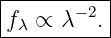 | (60) |
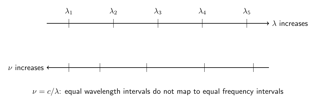
A spectrum that appears horizontal on an fν versus ν plot does not appear horizontal on an fλ versus λ plot.
Conversely, a spectrum flat in fλ is not flat in fν.
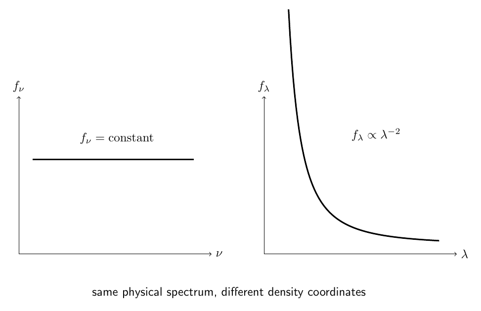
Figure 4. The same physical spectrum can have different plotted shapes in per-wavelength and per-frequency representations because the spectral density transforms with a wavelength-dependent Jacobian.
A blackbody can be represented by
 | (61) |
or
 | (62) |
These describe the same thermal radiation but are densities per different spectral coordinates.
Consequently, the maximum of
 | (63) |
does not correspond to the maximum of
 | (64) |
by simply substituting
 | (65) |
The wavelength-space and frequency-space density functions include the same Jacobian issue as fλ and fν.
This is why the phrase
 | (66) |
is incomplete unless the spectral representation is specified.
Because fλ is a density per unit wavelength, its numerical value changes when the wavelength unit changes.
Suppose
 | (67) |
is measured per meter.
Since
 | (68) |
the same physical spectrum expressed per nanometer satisfies
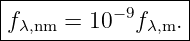 | (69) |
Similarly,
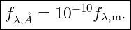 | (70) |
This factor is required because a one-nanometer bin is much narrower than a one-meter wavelength bin.
A commonly encountered cgs unit is
 | (71) |
The conversion is
 | (72) |
Equivalently,
 | (73) |
Careful unit labeling is essential when comparing spectra from different catalogs or instruments.
Frequency spectral flux density is commonly expressed in janskys.
The jansky is defined by
 | (74) |
In cgs units,
 | (75) |
Submultiples are common:
| 1 mJy | = 10−3 Jy, | (76) |
| 1 μJy | = 10−6 Jy, | (77) |
| 1 nJy | = 10−9 Jy. | (78) |
Radio astronomy commonly reports source flux densities directly in Jy, mJy, or smaller units.
Consider
 | (79) |
In SI,
 | (80) |
At
 | (81) |
| fλ | =  fν fν | (82) |
| ≈ 3.598 × 10⁻² W m−2 m−1. | (83) |
Per nanometer,
 | (84) |
Per angstrom in cgs units,
 | (85) |
This example demonstrates why a large numerical value in Jy can correspond to a small numerical value per nanometer or per angstrom.
The AB magnitude system is designed around frequency spectral flux density.
A source with constant
 | (86) |
has constant AB magnitude with frequency under the idealized monochromatic definition.
The conventional zero point corresponds approximately to
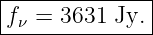 | (87) |
For a monochromatic flux density, one commonly writes
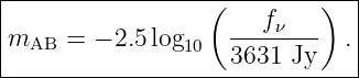 | (88) |
For real broadband observations, the instrument response and the precise averaging convention must be included.
Thus the 3631 Jy relation is an entry point to the AB system, not a substitute for full synthetic photometry.
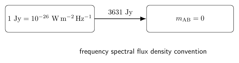
Figure 5. The jansky is a unit of frequency spectral flux density, and the AB magnitude convention is tied to a reference frequency flux density of approximately 3631 janskys.
A source can also be described intrinsically by its luminosity per unit wavelength or frequency.
Define
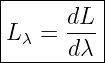 | (89) |
and
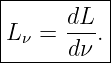 | (90) |
Their units are
| [Lλ] | = W m−1, | (91) |
| [Lν] | = W Hz−1. | (92) |
They satisfy the same coordinate transformation:
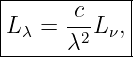 | (93) |
and
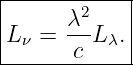 | (94) |
For an isotropic source in ordinary Euclidean geometry, with no absorption, redshift, or other propagation effects, the spectral luminosity density and observed spectral flux density satisfy
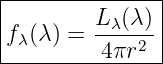 | (95) |
and
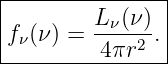 | (96) |
The total luminosity relation
 | (97) |
is therefore mirrored at each spectral coordinate.
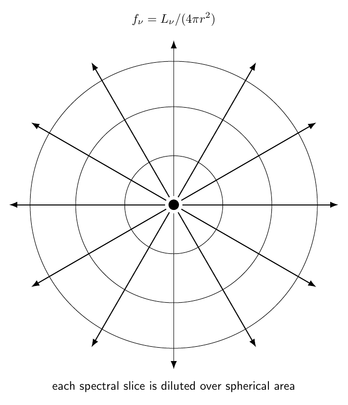
Figure 6. In the simple isotropic noncosmological case, every spectral slice of the luminosity spreads over the same spherical area, so spectral flux density also obeys inverse-square dilution.
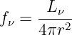
The simple relation
 | (98) |
assumes that source and observer use corresponding spectral coordinates without additional shifts.
Real observations can require corrections for:
In cosmology, observed and emitted frequency intervals differ by redshift factors, so the monochromatic luminosity-flux relation requires additional care.
The inverse-square expression above is therefore the correct introductory local relation, not a universal formula for every astronomical situation.
If the complete spectrum is known,
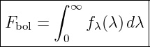 | (99) |
is the bolometric flux.
Equivalently,
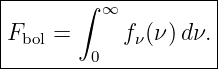 | (100) |
If only a finite spectral range is integrated, the result is a band-limited or interval-integrated flux.
For example,
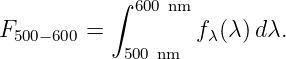 | (101) |
This distinction is central when comparing a detector measurement with a source’s bolometric output.
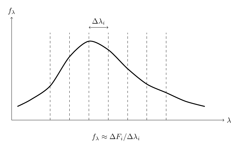
A real spectrograph produces measurements in finite bins or pixels.
If bin i has width
 | (102) |
and calibrated spectral flux density
 | (103) |
then the integrated flux can be approximated by
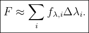 | (104) |
For nonuniform wavelength bins, each bin must use its own
 | (105) |
This discrete expression is the numerical counterpart of the continuous integral.
Many astronomical spectra contain both a smooth continuum and narrow spectral features.
Write schematically
 | (106) |
The integrated line flux is often obtained by subtracting the local continuum and integrating across the line:
![|---------------------------------|
| ∫ |
Fline = [fλ(λ ) − fλ,cont(λ)]dλ.|
---------line-----------------------](https://images.physicslibrary.org/cache/objects/1438/make4ht/SpectralFluxDensityDefinitionUnitsAndAstrophysicalUse99x.png) | (107) |
The line flux has ordinary flux units:
 | (108) |
even though the spectrum being integrated has spectral-flux-density units.
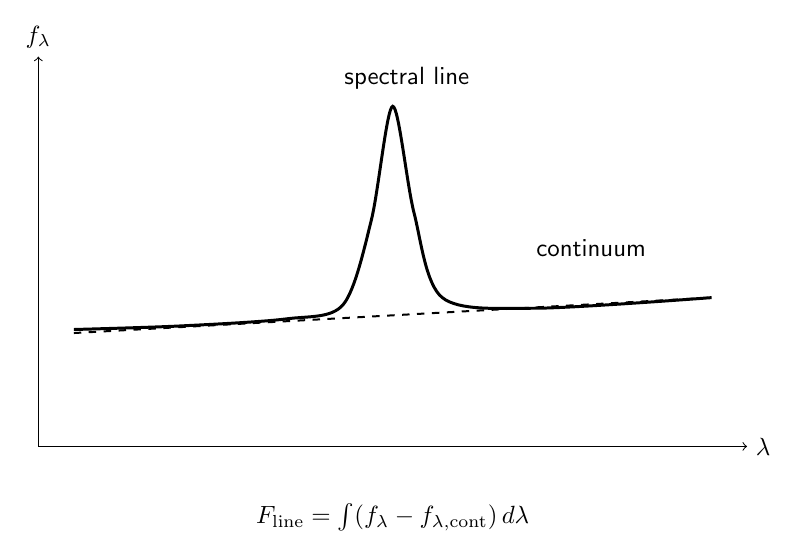
Figure 7. A spectral line sits above or below a local continuum. Integrating the continuum-subtracted spectral flux density across the feature gives an integrated line flux.
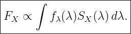
A broadband detector samples a weighted portion of the spectrum.
Let
 | (109) |
represent the response of photometric band X.
An energy-weighted schematic band signal is
 | (110) |
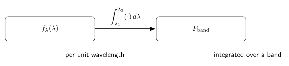
This is the equation that motivated the present article.
It says:
The measurement is therefore not generally equal to the spectrum evaluated at one representative wavelength.
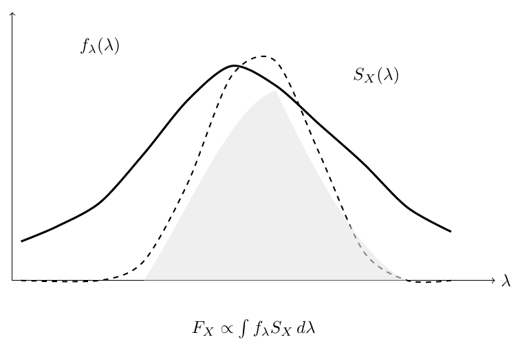
Figure 8. A photometric passband performs a weighted integration of the source spectral flux density across a finite wavelength range.
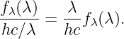
A photon-counting detector responds to photon number, not directly to radiant energy.
Each photon has energy
 | (111) |
Therefore a spectral energy flux density corresponds to a photon spectral rate proportional to
 | (112) |
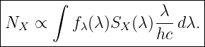
A schematic photon count rate is therefore
 | (113) |
Depending on the adopted convention, some or all of the photon-weighting factors may be absorbed into the published response function.
This is why photometric passband definitions must be read carefully.
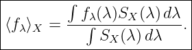
Sometimes the goal is not an integrated band flux but a representative band-averaged spectral flux density.
A simple energy-weighted wavelength average can have the schematic form
 | (114) |
Other photometric systems use different weightings and normalizations.
The important point is that an average spectral flux density requires both:
The next PhysicsLibrary article on photometric passbands and system response should develop these details more fully.
Several closely related quantities are easy to confuse.
 | (115) |
or
 | (116) |
describes received power per detector area per spectral interval.
 | (117) |
or
 | (118) |
describes intrinsic source power per spectral interval.
A quantity such as
 | (119) |
also retains directional information per unit solid angle.
A common SI unit is
 | (120) |
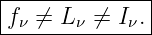
Thus
 | (121) |
They are related, but they answer different physical questions.
 to
to 
Suppose
 | (122) |
at
 | (123) |
First convert the density from per nanometer to per meter:
 | (124) |
Then
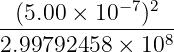
| fν | =  fλ fλ | (125) |
=  (1.00 × 10⁻²) (1.00 × 10⁻²) | (126) | |
| ≈ 8.34 × 10⁻²⁴ W m−2 Hz−1. | (127) |
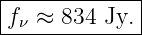
In janskys,
 | (128) |
The large-looking Jy number and the small per-nanometer number represent the same physical spectrum.
Suppose a calibrated spectrum has three adjacent 10 nm bins:
| Central wavelength | fλ | Bin width |
| 500 nm | 1.0 × 10⁻¹¹ | 10 nm |
| 510 nm | 1.4 × 10⁻¹¹ | 10 nm |
| 520 nm | 1.2 × 10⁻¹¹ | 10 nm |
with fλ in
 | (129) |
Approximate the integrated flux as
| F | ≈∑ ifλ,iΔλi | (130) |
= 10 × 10−11 × 10−11 | (131) | |
| = 3.6 × 10⁻¹⁰ W m−2. | (132) |
This is exactly the same logic as a Riemann sum.
Suppose an isotropic source has
 | (133) |
at some frequency, and it lies at
 | (134) |
Using
 | (135) |
the distance is
 | (136) |
Then
| fν | =  | (137) |
| ≈ 8.36 × 10⁻²³ W m−2 Hz−1. | (138) |
In janskys,
 | (139) |
The example illustrates that the inverse-square law applies to spectral luminosity density just as it applies to total luminosity in the simple noncosmological case.
The article Electromagnetic Waves and Wavelength: Frequency, Propagation, and Spectral Description supplies the relation
 | (140) |
and explains why wavelength and frequency are reciprocal spectral coordinates.
The electromagnetic spectrum article provides the larger band context in which spectral flux densities are measured.
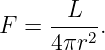
The Luminosity article distinguishes intrinsic luminosity from received flux and gives the inverse-square relation
 | (141) |
The present article extends that idea spectrally:
 | (142) |
under the simple local isotropic assumptions described above.
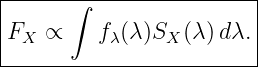
The article on Color in Astrophysics uses broadband measurements whose underlying source information is the spectral flux density.
The next natural bridge is the response-weighted integral
 | (143) |
Thus the conceptual chain is
 | (144) |
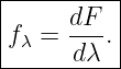
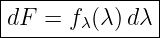
Spectral flux density describes how received electromagnetic flux is distributed across a spectral coordinate.
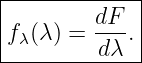
Per wavelength,
 | (145) |
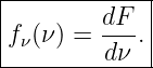
Per frequency,
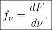 | (146) |
The total flux is
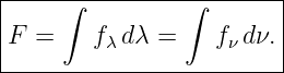 | (147) |
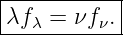
The two spectral densities are related by
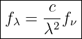 | (148) |
and
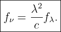 | (149) |
A particularly useful identity is
 | (150) |
Frequency spectral flux density is often quoted in janskys:
 | (151) |
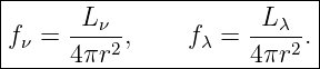
For a simple isotropic source,
 | (152) |
Finally, photometric measurements use weighted spectral integrals rather than a single wavelength value:
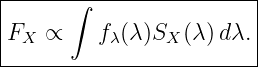 | (153) |
This is the key bridge from a physical spectrum to broadband astronomical photometry.
[1] G. B. Rybicki and A. P. Lightman, Radiative Processes in Astrophysics, Wiley, 1979.
[2] B. W. Carroll and D. A. Ostlie, An Introduction to Modern Astrophysics, 2nd ed., Pearson, 2007.
[3] D. W. Hogg, What is a magnitude?, arXiv:2206.00989.
[4] M. S. Bessell and S. J. Murphy, Spectrophotometric libraries, revised photonic passbands, and zero points for UBVRI, Hipparcos, and Tycho photometry, Publications of the Astronomical Society of the Pacific, 124, 140, 2012.
[5] J. B. Oke and J. E. Gunn, Secondary standard stars for absolute spectrophotometry, The Astrophysical Journal, 266, 713, 1983.
[6] D. W. Hogg, Distance measures in cosmology, arXiv:astro-ph/9905116.
| Also defines: | spectral flux density, flux density per wavelength, flux density per frequency, f_lambda, f_nu, jansky, band-integrated flux, spectral luminosity density |
| Keywords: | spectral flux density, spectral irradiance, f_lambda, f_nu, jansky, Jy, AB magnitude, spectrum, wavelength, frequency, photometry, passband, luminosity density, blackbody |
| Physics Classification: | 95.75.-z (Observation and data reduction techniques; computer modeling and simulation) |
| 42.25.Bs (Wave propagation, transmission and absorption radiation interactions with plasma and 52.38-r Laser-plasma interactions-in pla) |
None.
No messages.











![[F] = W m −2.](https://images.physicslibrary.org/cache/objects/1438/make4ht/SpectralFluxDensityDefinitionUnitsAndAstrophysicalUse16x.png)
![|------------------|
|[f λ] = W m −2m −1 |
-------------------](https://images.physicslibrary.org/cache/objects/1438/make4ht/SpectralFluxDensityDefinitionUnitsAndAstrophysicalUse17x.png)
![|-----------−2---−-1-|
-[fν] =-W-m----Hz--.-|](https://images.physicslibrary.org/cache/objects/1438/make4ht/SpectralFluxDensityDefinitionUnitsAndAstrophysicalUse18x.png)







 and
and 











 and
and 