
|
|
|
|||||||
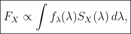
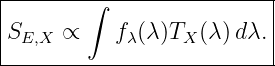
then the measured band signal is constructed from a weighted integral across wavelength. A schematic energy-weighted form is
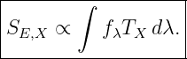
where X labels the photometric band and SX(λ) describes the system response. For a photon-counting detector, an additional photon-number weighting appears unless it has already been absorbed into the published response curve. This article develops what a passband means, what belongs inside a system response, why different detector conventions produce different weighting factors, and how a source spectrum is converted into a synthetic photometric measurement.
1 Why a photometric band is not one wavelengthA broadband filter such as B, V , g, r, or G accepts light over a finite spectral interval. Even if one associates a band with a nominal wavelength such as
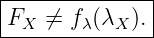
the detector generally receives photons from a broad neighborhood around that wavelength. Therefore, in general,
The measured signal depends on:
A representative or effective wavelength can be useful, but it does not replace the full passband integral.
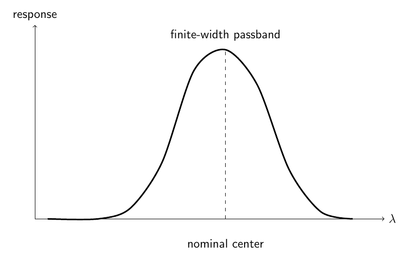
Figure 1. A photometric passband admits a finite wavelength range with varying efficiency rather than sampling only one wavelength.
2 Transmission, response, and throughputThe words transmission, response, and throughput are related but should not automatically be treated as identical. A filter transmission curve,
describes the fraction of incident radiation transmitted by the filter. A detector quantum efficiency,
describes the fraction of incident photons that produce detected charge carriers or recorded events, under an appropriate detector model. A telescope or optical train has its own wavelength-dependent efficiency,
For a ground-based observation, atmospheric transmission may contribute
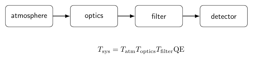
A simple total throughput can therefore be represented schematically by
Additional components can be included when necessary. The product form reflects a sequence of efficiencies: radiation must survive or be detected by every stage of the system.
Figure 2. A total system throughput can combine atmosphere, telescope optics, filter transmission, and detector sensitivity into one wavelength-dependent response.
3 Absolute versus relative responseA response curve may be calibrated absolutely, or it may be normalized to an arbitrary peak such as
For many synthetic-photometry calculations, only the shape of the response matters because an overall multiplicative constant cancels when the signal is normalized or compared with a reference source. If
then
A corresponding zero point or normalization can absorb C. However, an absolute detector count-rate prediction requires an absolute throughput calibration together with collecting area, exposure time, and detector gain or event efficiency as appropriate.
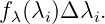
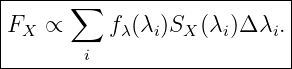
4 The weighted-integral pictureSuppose the wavelength axis is divided into narrow bins. In bin i, the source contributes approximately
If the system response in that bin is
the weighted contribution is approximately
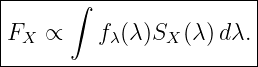
Adding the bins gives
Taking the continuum limit gives Equation (1):
Thus the passband measurement is a continuous weighted sum over the spectrum.
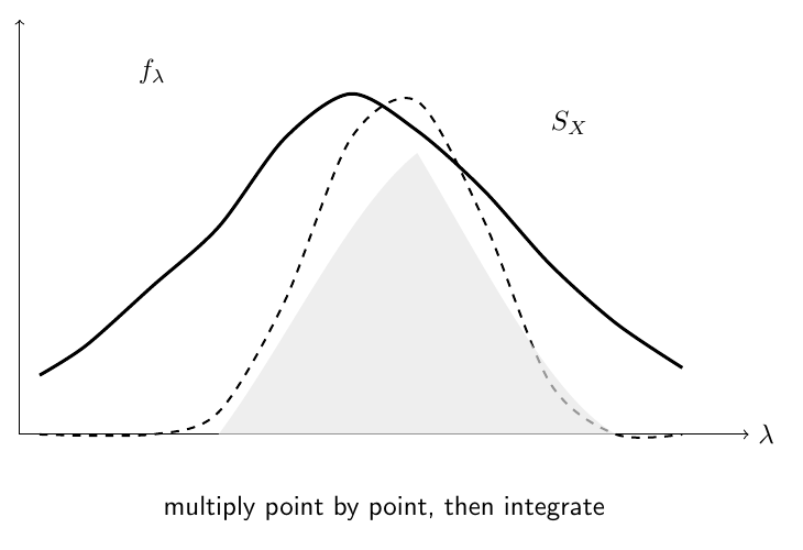
Figure 3. The source spectrum is multiplied wavelength by wavelength by the system response, and the weighted contributions are integrated across the passband.
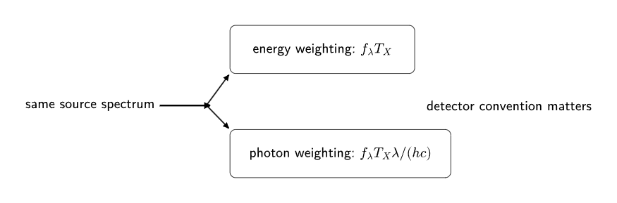
5 Energy-measuring and photon-counting detectorsEquation (5) is a useful schematic expression, but the correct weighting depends on what the detector measures. An idealized energy-measuring detector responds in proportion to radiant energy deposited. For such a convention,
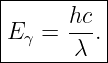
A photon-counting detector responds approximately to the number of detected photons. A photon at wavelength λ has energy
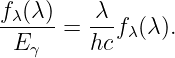
The incident photon spectral rate per detector area is therefore proportional to
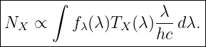
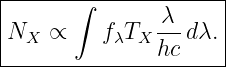
Thus a photon-counting signal has the schematic form
The factor
converts radiant energy into photon number.
Figure 4. Energy weighting and photon counting are not identical because a photon carries energy inversely proportional to wavelength.
6 Why published response curves must be read carefullySome published passband curves represent physical throughput
before photon-number weighting. Other published response functions are defined so that detector behavior is already incorporated into
Therefore one must not automatically multiply every published passband by an additional factor of λ. The correct procedure is:
This convention dependence is one reason that synthetic photometry should be based on the documented system response rather than only on a filter name.
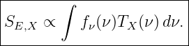
7 Frequency-space formThe same measurement can be written in frequency coordinates. For an energy-weighted response,
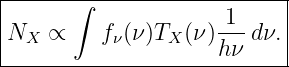
For photon counting,
The wavelength and frequency expressions are equivalent when the spectral densities, response functions, and integration measures are transformed consistently.
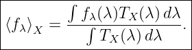
8 Normalized band averagesSometimes one wants a representative spectral flux density rather than an unnormalized integrated signal. For an energy-weighted wavelength response, a simple normalized mean is
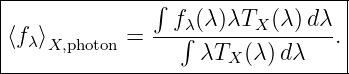
For a photon-counting response described by a physical throughput TX(λ),
These are weighted averages. Different photometric systems can define band averages differently, so the response convention remains part of the definition.
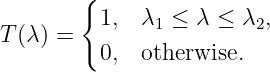
9 A simple top-hat passbandAn ideal top-hat response is
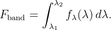
For energy weighting,
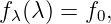
If fλ is constant,
then
This idealized example makes the role of finite bandwidth explicit.
10 Example 1: energy-weighted top-hat bandSuppose
and
is constant across the band. Then
The band flux depends on both the spectral density and the width of the accepted wavelength interval.
11 Basic passband descriptorsSeveral different numbers are used to summarize a passband. They do not all mean the same thing. Useful descriptors include:
No single number contains all of the information in the full response curve.
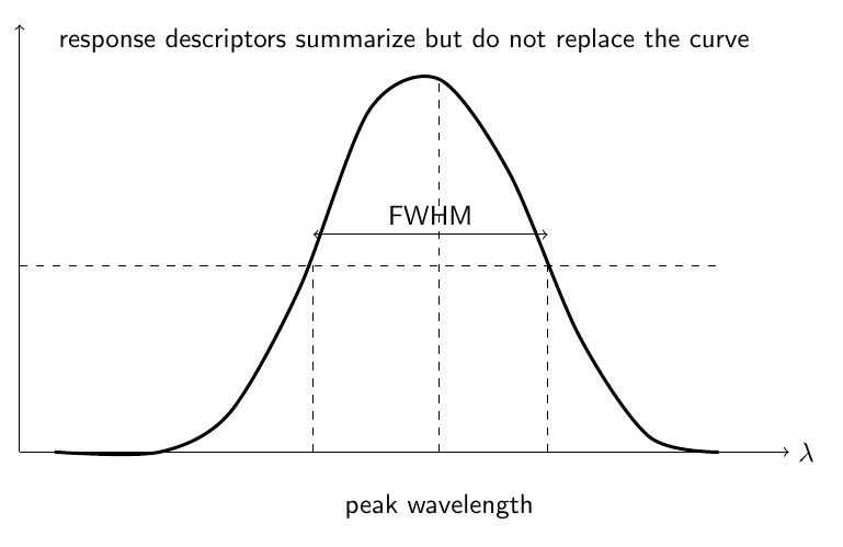
Figure 5. A passband can be summarized by several characteristic wavelengths and widths, but these descriptors do not replace the complete response function.
12 Wavelength of maximum responseThe wavelength of maximum response is simply the location at which
is largest. If the response has multiple peaks or a flat plateau, even this quantity may not be unique or especially informative. It depends only on the response curve, not on the source spectrum.
13 Full width at half maximumIf the response has a single well-defined peak, the full width at half maximum is the wavelength separation between the two points at which the response equals half the peak value. Symbolically,
The full width at half maximum is useful for simple, roughly bell-shaped passbands but can be misleading for asymmetric or multi-peaked responses.
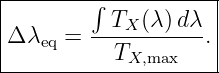
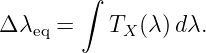
14 Equivalent rectangular bandwidthA useful response-only width is the equivalent rectangular bandwidth,
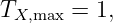
If the response is normalized so that
then
This is the width of a rectangle with height equal to the peak response and area equal to the area under the actual response curve.
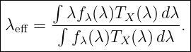
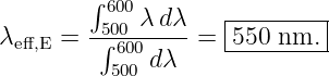
15 Effective wavelengthAn effective wavelength is intended to represent the wavelength at which a particular source and response combination is concentrated. A common energy-weighted form is
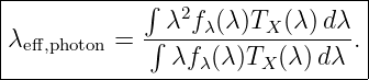
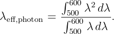
For photon weighting, the corresponding source weighting changes because the detected photon rate contains an additional factor of λ. For example,
The key conceptual point is:
A red star and a blue star observed through the same broad filter can therefore have different effective wavelengths.
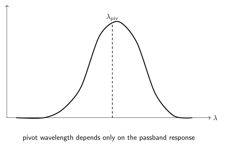
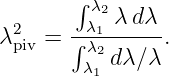
16 Pivot wavelengthThe pivot wavelength is designed to characterize the passband itself rather than a particular source spectrum. For a dimensionless throughput TX(λ), the commonly used definition is
Unlike an effective wavelength,
It is especially useful when converting consistently between appropriately defined band-averaged fλ and fν quantities.
Figure 6. Pivot wavelength is a property of the response curve, whereas effective wavelength usually also depends on the spectrum of the observed source.
17 Example 2: pivot wavelength of an ideal top-hat bandFor
between λ1 and λ2,
Therefore
For
This value is close to, but not defined simply as, the arithmetic midpoint of the band.
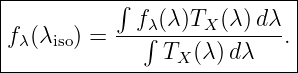
18 Isophotal wavelengthAn isophotal wavelength is defined so that the monochromatic spectral flux density at that wavelength equals a suitable band-averaged spectral flux density. For an energy-weighted convention, one may define λiso through
Because the left side depends on the source spectrum, the isophotal wavelength is generally source dependent. For some spectra and complex passbands, there can be more than one wavelength satisfying the equality. Therefore isophotal wavelength should not be confused with a universal center of the filter.
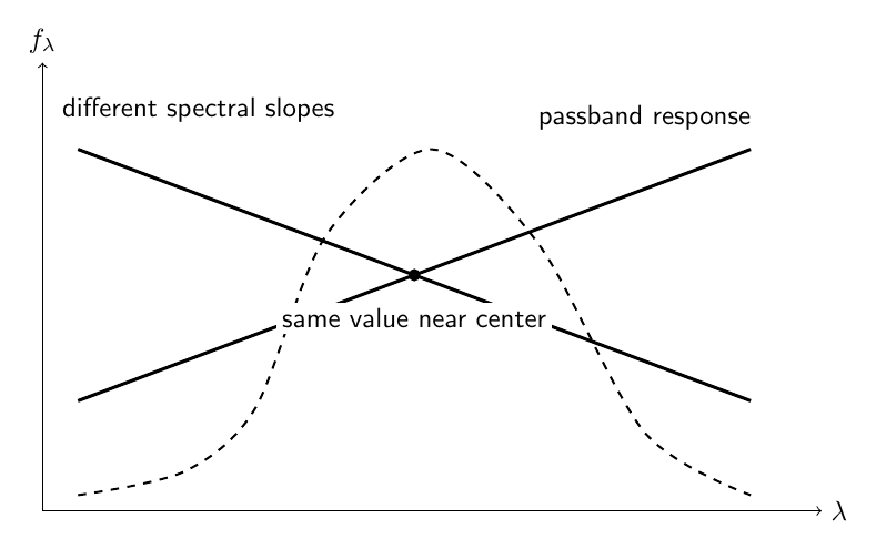
19 Two sources can agree at one wavelength and disagree in the bandSuppose two source spectra satisfy
at the nominal band center. If one spectrum rises toward the red while the other falls, then generally
Thus equality at one wavelength does not imply equality of broadband photometric signal.
Figure 7. Two spectra can cross at a nominal central wavelength yet produce different integrated signals because their shapes differ across the rest of the passband.
20 Synthetic photometrySynthetic photometry predicts a photometric measurement from a calibrated spectrum and a documented system response. The general procedure is:
Symbolically, define a detector signal functional
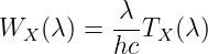
where WX includes the response and the detector-specific weighting. For example,
for a simple energy-weighted convention, while
for a simple photon-counting convention.
Figure 8. Synthetic photometry combines a calibrated source spectrum, a documented system response, the correct detector weighting, and a photometric reference or zero point.
21 From a synthetic signal to a magnitudeA magnitude is logarithmic. A general calibrated form can be written as
where ZPX is the zero point appropriate to the signal convention and units. Equivalently, relative to a reference source,
The reference spectrum and response convention are part of the definition of the photometric system.
22 AB, ST, and Vega-based systemsDifferent magnitude systems use different reference conventions.
AB systemThe AB system is tied to frequency spectral flux density. Its monochromatic definition can be expressed relative to approximately
Broadband AB magnitudes require the appropriate passband-weighted treatment rather than evaluation at one arbitrary wavelength.
ST systemThe ST system is formulated so that a source with constant
has constant ST magnitude under the corresponding convention.
Vega-based systemsVega-based systems use the spectrum of Vega, or a defined realization of that reference, to establish photometric zero points. Therefore the same instrumental bandpass can produce different numerical magnitude zero points depending on the adopted magnitude system.
23 Color indicesAn astronomical color is a difference of magnitudes:
Since each magnitude is derived from a different weighted passband integral,
the color measures how the source spectrum is distributed relative to the two response functions. This explains why astronomical color is not equivalent to assigning a single visible wavelength to the source.
24 Atmospheric responseFor ground-based photometry, the atmosphere can be an important part of the effective system response. Transmission depends on:
Thus one may distinguish:
from
A photometric standard system may then require transformations from the natural instrumental system to a defined standard system.
25 Red leaks and out-of-band responseA response curve need not vanish perfectly outside its nominal wavelength range. A small unintended transmission feature at longer wavelengths is often called a red leak. Likewise, unwanted sensitivity can occur on the blue side or elsewhere. Even a weak leak can matter if the source spectrum is much brighter in the leak region than inside the nominal passband. Therefore
can produce a non-negligible signal. This is another reason to use the full measured system response rather than an idealized central wavelength and width.
26 Example 3: same central flux, different broadband signalsConsider an ideal top-hat band from
to
Let the nominal center be
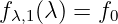
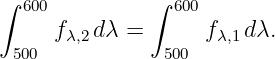
Suppose two spectra have the same value
at 550 nm. Let
and
If the top-hat band is perfectly symmetric about 550 nm, the linear positive and negative slope contributions cancel in an energy-weighted integral:
This special cancellation is a useful warning: the outcome depends on both the source spectrum and the response shape. For an asymmetric real passband, or for nonlinear spectral curvature, equality at the nominal center does not generally imply equal integrated signal. For photon counting, the extra factor of λ can also break the symmetry even for this simple linear example.
27 Example 4: photon weighting shifts the mean wavelengthConsider the same ideal top-hat band from 500 to 600 nm and a source with constant fλ. For energy weighting, the effective wavelength is the arithmetic mean:
For photon weighting,
Therefore
Longer-wavelength photons carry less energy individually, so a fixed spectral energy flux corresponds to more photons at longer wavelength.
28 Calibration and zero pointsA real photometric measurement does not end with the raw integral. Calibration must account for quantities such as:
The response integral tells how the source spectrum maps into an instrumental signal. The calibration procedure then maps that instrumental signal into a reproducible photometric quantity.
29 Common mistakes
30 Connections to other PhysicsLibrary articlesThe article Electromagnetic Waves and Wavelength establishes wavelength and frequency as spectral coordinates:
The article Spectral Flux Density defines
and
The present article adds the instrument response and produces the weighted band signal:
The article Color in Astrophysics then compares two such band measurements through
Thus the full conceptual chain is
31 SummaryA photometric passband describes wavelength-dependent sensitivity over a finite spectral interval. A total system throughput can combine several multiplicative components:
For an energy-weighted convention,
For a photon-counting convention based on a physical throughput,
An effective wavelength is generally source dependent, while the pivot wavelength
is a property of the response curve itself. Synthetic photometry can be summarized by
followed by a calibrated magnitude relation such as
The central lesson is that a broadband photometric measurement is an integral over the source spectrum and the complete system response, not a monochromatic measurement at a single wavelength.
References
References
[1] M. S. Bessell and S. J. Murphy, Spectrophotometric libraries, revised photonic passbands, and zero points for UBVRI, Hipparcos, and Tycho photometry, Publications of the Astronomical Society of the Pacific, 124, 140, 2012. [2] D. W. Hogg, What is a magnitude?, arXiv:2206.00989. [3] J. B. Oke and J. E. Gunn, Secondary standard stars for absolute spectrophotometry, The Astrophysical Journal, 266, 713, 1983. [4] M. S. Bessell, Standard photometric systems, Annual Review of Astronomy and Astrophysics, 43, 293, 2005. [5] G. B. Rybicki and A. P. Lightman, Radiative Processes in Astrophysics, Wiley, 1979. [6] B. W. Carroll and D. A. Ostlie, An Introduction to Modern Astrophysics, 2nd ed., Pearson, 2007. "Photometric Passbands and System Response: Throughput, Weighting, and Synthetic Photometry" is owned by bloftin.
Cross-references: relation, Jacobian, color, units, magnitude, flux, functions, energy, system, charge, radiation, calibration, light, spectral flux density, detect, telescope, spectrum There is 1 reference to this object. This is version 1 of Photometric Passbands and System Response: Throughput, Weighting, and Synthetic Photometry, born on 2026-10-08. Object id is 1439, canonical name is PhotometricPassbandsAndSystemResponseThroughputWeightingAndSyntheticPhotometry. Accessed 9 times total. Classification:
|
|
|
|
Pending Errata and AddendaNone.
|
DiscussionNo messages.
|
Interact |


















![|------[-∫------------]----|
| λTX (λ) dλ 1∕2 |
|λpiv = ∫------------- .|
-----------TX(λ-)dλ∕λ-------](https://images.physicslibrary.org/cache/objects/1439/make4ht/PhotometricPassbandsAndSystemResponseThroughputWeightingAndSyntheticPhotometry41x.png)


![|------------------------|
| [ λ2− λ2 ]1∕2 |
|λpiv = ---2----1-- .|
---------2ln(λ2∕λ1-)-----|](https://images.physicslibrary.org/cache/objects/1439/make4ht/PhotometricPassbandsAndSystemResponseThroughputWeightingAndSyntheticPhotometry45x.png)



![|--------∫-----------------|
| |
𝒮X [f] = fλ(λ)WX (λ )dλ,|
----------------------------](https://images.physicslibrary.org/cache/objects/1439/make4ht/PhotometricPassbandsAndSystemResponseThroughputWeightingAndSyntheticPhotometry50x.png)


![|------------------------------|
-mX--=-−-2.5log10𝒮X-[f] +-ZPX-,-](https://images.physicslibrary.org/cache/objects/1439/make4ht/PhotometricPassbandsAndSystemResponseThroughputWeightingAndSyntheticPhotometry53x.png)
![|-------------------------[--------]-|
m − m = − 2.5 log -𝒮X-[f-]- .|
| X X,ref 10 𝒮X [fref] |
--------------------------------------](https://images.physicslibrary.org/cache/objects/1439/make4ht/PhotometricPassbandsAndSystemResponseThroughputWeightingAndSyntheticPhotometry54x.png)



![mX ← − 𝒮X [f], mY ← − 𝒮Y [f],](https://images.physicslibrary.org/cache/objects/1439/make4ht/PhotometricPassbandsAndSystemResponseThroughputWeightingAndSyntheticPhotometry58x.png)





![[ λ − 550 nm ]
fλ,2(λ) = f0 1 + a------------ .
50 nm](https://images.physicslibrary.org/cache/objects/1439/make4ht/PhotometricPassbandsAndSystemResponseThroughputWeightingAndSyntheticPhotometry67x.png)



![|----------------------------------|
-fλ(λ)---+---SX-(λ)---−→----𝒮X-[f].-](https://images.physicslibrary.org/cache/objects/1439/make4ht/PhotometricPassbandsAndSystemResponseThroughputWeightingAndSyntheticPhotometry75x.png)



![|------[-∫---------]1∕2|
| --λTX--dλ-- |
|λpiv = ∫ T dλ∕λ |
------------X-----------](https://images.physicslibrary.org/cache/objects/1439/make4ht/PhotometricPassbandsAndSystemResponseThroughputWeightingAndSyntheticPhotometry81x.png)
![|--------∫-----------------|
| |
𝒮X [f] = fλ(λ)WX (λ )dλ,|
----------------------------](https://images.physicslibrary.org/cache/objects/1439/make4ht/PhotometricPassbandsAndSystemResponseThroughputWeightingAndSyntheticPhotometry82x.png)
![|------------------------------|
-mX--=-−-2.5log10𝒮X-[f] +-ZPX-.-](https://images.physicslibrary.org/cache/objects/1439/make4ht/PhotometricPassbandsAndSystemResponseThroughputWeightingAndSyntheticPhotometry83x.png)