At about the time that Galileo was beginning his experiments with falling bodies, the efforts of two
other scientists dramatically advanced our understanding of the motions of the planets. These two
astronomers were the observer Tycho Brahe and the mathematician Johannes Kepler. Together,
they placed the speculations of Copernicus on a sound mathematical basis and paved the way for
the work of Isaac Newton in the next century.
Tycho Brahe’s Observatory
Three years after the publication of Copernicus’ De Revolutionibus, Tycho Brahe was born to a
family of Danish nobility. He developed an early interest in astronomy and, as a young
man, made significant astronomical observations. Among these was a careful study of
what we now know was an exploding star that flared up to great brilliance in the night
sky.
His growing reputation gained him the patronage of the Danish King Frederick II, and at the age
of 30, Brahe was able to establish a fine astronomical observatory on the North Sea island of
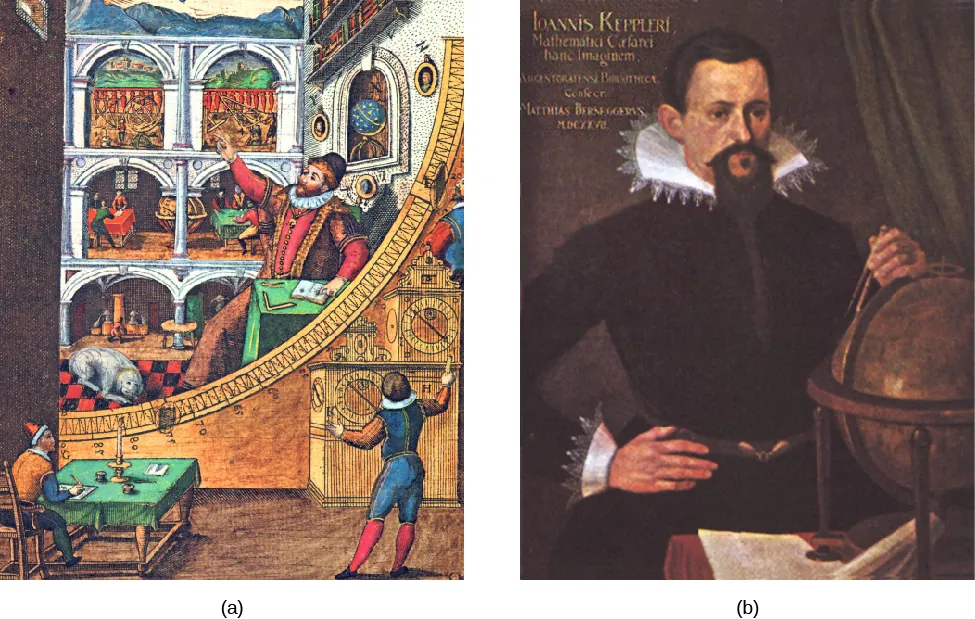
Hven (Figure 3.2). Brahe was the last and greatest of the pre-telescopic observers in
Europe.
Figure 3.2 Tycho Brahe (1546–1601) and Johannes Kepler (1571–1630). (a) A stylized engraving
shows Tycho Brahe using his instruments to measure the altitude of celestial objects above the
horizon. The large curved instrument in the foreground allowed him to measure precise angles in
the sky. Note that the scene includes hints of the grandeur of Brahe’s observatory at Hven. (b)
Kepler was a German mathematician and astronomer. His discovery of the basic laws that describe
planetary motion placed the heliocentric cosmology of Copernicus on a firm mathematical
basis.
At Hven, Brahe made a continuous record of the positions of the Sun, Moon, and planets
for almost 20 years. His extensive and precise observations enabled him to note that
the positions of the planets varied from those given in published tables, which were
based on the work of Ptolemy. These data were extremely valuable, but Brahe didn’t
have the ability to analyze them and develop a better model than what Ptolemy had
published.
He was further inhibited because he was an extravagant and cantankerous fellow, and he
accumulated enemies among government officials. When his patron, Frederick II, died in 1597,
Brahe lost his political base and decided to leave Denmark. He took up residence in Prague, where
he became court astronomer to Emperor Rudolf of Bohemia. There, in the year before his death,
Brahe found a most able young mathematician, Johannes Kepler, to assist him in analyzing his
extensive planetary data.
Johannes Kepler
Johannes Kepler was born into a poor family in the German province of Württemberg and lived
much of his life amid the turmoil of the Thirty Years’ War (see Figure 3.2). He attended university
at Tubingen and studied for a theological career. There, he learned the principles of the
Copernican system and became converted to the heliocentric hypothesis.
Eventually, Kepler went to Prague to serve as an assistant to Brahe, who set him to work trying to
find a satisfactory theory of planetary motion—one that was compatible with the long series of
observations made at Hven. Brahe was reluctant to provide Kepler with much material at any one
time for fear that Kepler would discover the secrets of the universal motion by himself, thereby
robbing Brahe of some of the glory. Only after Brahe’s death in 1601 did Kepler get full possession
of the priceless records. Their study occupied most of Kepler’s time for more than 20
years.
Through his analysis of the motions of the planets, Kepler developed a series of principles, now
known as Kepler’s three laws, which described the behavior of planets based on their paths
through space. The first two laws of planetary motion were published in 1609 in The
New Astronomy. Their discovery was a profound step in the development of modern
science.
The First Two Laws of Planetary Motion
The path of an object through space is called its orbit. Kepler initially assumed that the orbits of
planets were circles, but doing so did not allow him to find orbits that were consistent with Brahe’s
observations. Working with the data for Mars, he eventually discovered that the orbit of that
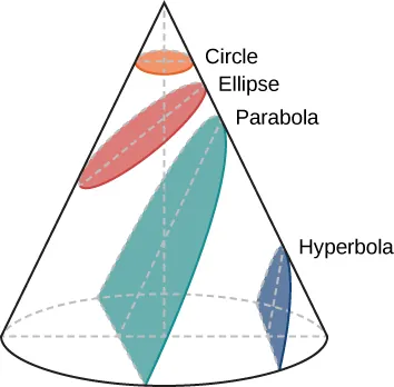
planet had the shape of a somewhat flattened circle, or ellipse. Next to the circle, the ellipse is the
simplest kind of closed curve, belonging to a family of curves known as conic sections (Figure
3.3).
Figure 3.3 Conic Sections. The circle, ellipse, parabola, and hyperbola are all formed
by the intersection of a plane with a cone. This is why such curves are called conic
sections.
You might recall from math classes that in a circle, the center is a special point. The distance from
the center to anywhere on the circle is exactly the same. In an ellipse, the sum of the distance from
two special points inside the ellipse to any point on the ellipse is always the same. These two points
inside the ellipse are called its foci (singular: focus), a word invented for this purpose by
Kepler.
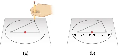
This property suggests a simple way to draw an ellipse (Figure 3.4). We wrap the ends of a loop of
string around two tacks pushed through a sheet of paper into a drawing board, so that
the string is slack. If we push a pencil against the string, making the string taut, and
then slide the pencil against the string all around the tacks, the curve that results is an
ellipse.
At any point where the pencil may be, the sum of the distances from the pencil to the two
tacks is a constant length—the length of the string. The tacks are at the two foci of the
ellipse.
The widest diameter of the ellipse is called its major axis. Half this distance—that is,
the distance from the center of the ellipse to one end—is the semimajor axis, which is
usually used to specify the size of the ellipse. For example, the semimajor axis of the
orbit of Mars, which is also the planet’s average distance from the Sun, is 228 million
kilometers.
Figure 3.4 Drawing an Ellipse. (a) We can construct an ellipse by pushing two tacks (the white
objects) into a piece of paper on a drawing board, and then looping a string around the tacks.
Each tack represents a focus of the ellipse, with one of the tacks being the Sun. Stretch the string
tight using a pencil, and then move the pencil around the tacks. The length of the string remains
the same, so that the sum of the distances from any point on the ellipse to the foci is always
constant. (b) In this illustration, each semimajor axis is denoted by a. The distance 2a is called the
major axis of the ellipse.
The shape (roundness) of an ellipse depends on how close together the two foci are, compared with
the major axis. The ratio of the distance between the foci to the length of the major axis is called
the eccentricity of the ellipse.
If the foci (or tacks) are moved to the same location, then the distance between the foci would be
zero. This means that the eccentricity is zero and the ellipse is just a circle; thus, a circle can
be called an ellipse of zero eccentricity. In a circle, the semimajor axis would be the
radius.
Next, we can make ellipses of various elongations (or extended lengths) by varying the spacing of
the tacks (as long as they are not farther apart than the length of the string). The greater the
eccentricity, the more elongated is the ellipse, up to a maximum eccentricity of 1.0, when the
ellipse becomes “flat,” the other extreme from a circle.
The size and shape of an ellipse are completely specified by its semimajor axis and
its eccentricity. Using Brahe’s data, Kepler found that Mars has an elliptical orbit,
with the Sun at one focus (the other focus is empty). The eccentricity of the orbit of
Mars is only about 0.1; its orbit, drawn to scale, would be practically indistinguishable
from a circle, but the difference turned out to be critical for understanding planetary
motions.
Kepler generalized this result in his first law and said that the orbits of all the planets are ellipses.
Here was a decisive moment in the history of human thought: it was not necessary to have only
circles in order to have an acceptable cosmos. The Universe could be a bit more complex than the
Greek philosophers had wanted it to be.
Kepler’s second law deals with the speed with which each planet moves along its ellipse, also
known as its orbital speed. Working with Brahe’s observations of Mars, Kepler discovered that the
planet speeds up as it comes closer to the Sun and slows down as it pulls away from the Sun. He
expressed the precise form of this relationship by imagining that the Sun and Mars are connected
by a straight, elastic line.
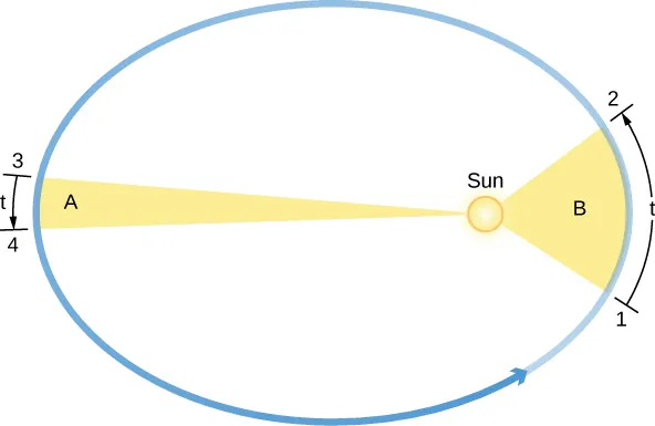
When Mars is closer to the Sun (positions 1 and 2 in Figure 3.5), the elastic line is not stretched as
much, and the planet moves rapidly. Farther from the Sun, as in positions 3 and 4, the line is
stretched a lot, and the planet does not move so fast. As Mars travels in its elliptical orbit around
the Sun, the elastic line sweeps out areas of the ellipse as it moves (the colored regions in our
figure). Kepler found that in equal intervals of time (t), the areas swept out in space by this
imaginary line are always equal; that is, the area of the region B from 1 to 2 is the same as that of
region A from 3 to 4.
If a planet moves in a circular orbit, the elastic line is always stretched the same amount and the
planet moves at a constant speed around its orbit. But, as Kepler discovered, in most orbits that
speed of a planet orbiting its star (or moon orbiting its planet) tends to vary because the orbit is
elliptical.
Figure 3.5 Kepler’s Second Law: The Law of Equal Areas. The orbital speed of a planet traveling
around the Sun (the circular object inside the ellipse) varies in such a way that in equal intervals of
time (t), a line between the Sun and a planet sweeps out equal areas (A and B). Note that the
eccentricities of the planets’ orbits in our solar system are substantially less than shown
here.
Link to Learning
The Kepler’s Second Law demonstrator (https://openstax.org/l/30kepsecond) from CCNY’s
ScienceSims project shows how an orbiting planet sweeps out the same area in the same
time.
Kepler’s Third Law
Kepler’s first two laws of planetary motion describe the shape of a planet’s orbit and allow
us to calculate the speed of its motion at any point in the orbit. Kepler was pleased
to have discovered such fundamental rules, but they did not satisfy his quest to fully
understand planetary motions. He wanted to know why the orbits of the planets were
spaced as they are and to find a mathematical pattern in their movements—a “harmony
of the spheres” as he called it. For many years he worked to discover mathematical
relationships governing planetary spacing and the time each planet took to go around the
Sun.
In 1619, Kepler discovered a basic relationship to relate the planets’ orbits to their relative
distances from the Sun. We define a planet’s orbital period, (P), as the time it takes a planet to
travel once around the Sun. Also, recall that a planet’s semimajor axis, a, is equal to its average
distance from the Sun. The relationship, now known as Kepler’s third law, says that a
planet’s orbital period squared is proportional to the semimajor axis of its orbit cubed,
or
When P (the orbital period) is measured in years, and a is expressed in a quantity known as an
astronomical unit (AU), the two sides of the formula are not only proportional but equal. One AU
is the average distance between Earth and the Sun and is approximately equal to 1.5 × 10⁸
kilometers. In these units,
Kepler’s third law applies to all objects orbiting the Sun, including Earth, and provides a
means for calculating their relative distances from the Sun from the time they take
to orbit. Let’s look at a specific example to illustrate how useful Kepler’s third law
is.
For instance, suppose you time how long Mars takes to go around the Sun (in Earth years).
Kepler’s third law can then be used to calculate Mars’ average distance from the Sun. Mars’ orbital
period (1.88 Earth years) squared, or P2, is 1.882 = 3.53, and according to the equation for
Kepler’s third law, this equals the cube of its semimajor axis, or a3. So what number must be
cubed to give 3.53? The answer is 1.52 (since 1.52 × 1.52 × 1.52 = 3.53). Thus, Mars’ semimajor
axis in astronomical units must be 1.52 AU. In other words, to go around the Sun in a little less
than two years, Mars must be about 50% (half again) as far from the Sun as Earth
is.
Kepler’s three laws of planetary motion can be summarized as follows:
- Kepler’s first law: Each planet moves around the Sun in an orbit that is an ellipse,
with the Sun at one focus of the ellipse.
- Kepler’s second law: The straight line joining a planet and the Sun sweeps out equal
areas in space in equal intervals of time.
- Kepler’s third law: The square of a planet’s orbital period is directly proportional to
the cube of the semimajor axis of its orbit.
Kepler’s three laws provide a precise geometric description of planetary motion within the
framework of the Copernican system. With these tools, it was possible to calculate planetary
positions with greatly improved precision. Still, Kepler’s laws are purely descriptive: they do not
help us understand what forces of nature constrain the planets to follow this particular set of rules.
That step was left to Isaac Newton.
Link to Learning
In honor of the scientist who first devised the laws that govern the motions of planets, the team
that built the first spacecraft to search for planets orbiting other stars decided to name the probe
“Kepler.” Visit NASA’s Kepler website to learn more about Johannes Kepler’s life and his laws of
planetary motion. NASA’s Kepler website (https://openstax.org/l/30nasakepmiss) and follow the
links that interest you.
Attribution
Access for free at openstax.org.
Bibliography
This entry is a derivative work of the original March 9, 2022 release identified in [1].
[1] Andrew Fraknoi, David Morrison, and Sidney C. Wolff, Astronomy 2e. Houston, Texas:
OpenStax, March 9, 2022. Digital ISBN 978-1-951693-50-3. Textbook content produced by
OpenStax in this edition is licensed under the Creative Commons Attribution 4.0 International
License (CC BY 4.0), except where otherwise noted. Changes: converted to LaTeX for
PhysicsLibrary and numbered worked examples separated into standalone entries. Access for free
at openstax.org.