0.1 Gaussian Co-Ordinates

From Relativity: The Special and General Theory by Albert Einstein

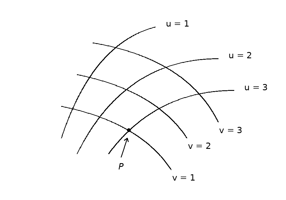
According to Gauss, this combined analytical and geometrical mode of handling the problem can be arrived at in the following way. We imagine a system of arbitrary curves (see Fig. 1) drawn on the surface of the table. These we designate as u-curves, and we indicate each of them by means of a number. The curves u = 1, u = 2 and u = 3 are drawn in the diagram. Between the curves u = 1 and u = 2 we must imagine an infinitely large number to be drawn, all of which correspond to real numbers lying between 1 and 2. fig. 04 We have then a system of u-curves, and this “infinitely dense” system covers the whole surface of the table. These u-curves must not intersect each other, and through each point of the surface one and only one curve must pass. Thus a perfectly definite value of u belongs to every point on the surface of the marble slab. In like manner we imagine a system of v-curves drawn on the surface. These satisfy the same conditions as the u-curves, they are provided with numbers in a corresponding manner, and they may likewise be of arbitrary shape. It follows that a value of u and a value of v belong to every point on the surface of the table. We call these two numbers the co-ordinates of the surface of the table (Gaussian co-ordinates). For example, the point P in the diagram has the Gaussian co-ordinates u = 3, v = 1. 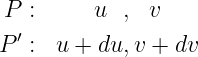Two neighbouring points P and P₁ on the surface then correspond to the co-ordinates

where du and dv signify very small numbers. In a similar manner we may indicate the distance (line-interval) between P and P₁, as measured with a little rod, by means of the very small number ds. Then according to Gauss we have

where g₁₁,g₁₂,g₂₂, are magnitudes which depend in a perfectly definite way on u and v. The magnitudes g₁₁, g₁₂ and g₂₂, determine the behaviour of the rods relative to the u-curves and v-curves, and thus also relative to the surface of the table. For the case in which the points of the surface considered form a Euclidean continuum with reference to the measuring-rods, but only in this case, it is possible to draw the u-curves and v-curves and to attach numbers to them, in such a manner, that we simply have:

Under these conditions, the u-curves and v-curves are straight lines in the sense of Euclidean geometry, and they are perpendicular to each other. Here the Gaussian coordinates are simply Cartesian ones. It is clear that Gauss co-ordinates are nothing more than an association of two sets of numbers with the points of the surface considered, of such a nature that numerical values differing very slightly from each other are associated with neighbouring points “in space.”

So far, these considerations hold for a continuum of two dimensions. But the Gaussian method can be applied also to a continuum of three, four or more dimensions. If, for instance, a continuum of four dimensions be supposed available, we may represent it in the following way. With every point of the continuum, we associate arbitrarily four numbers, x₁,x₂,x₃,x₄, which are known as “co-ordinates.” Adjacent points correspond to adjacent values of the coordinates. If a distance ds is associated with the adjacent points P and P₁, this distance being measurable and well defined from a physical point of view, then the following formula holds:

where the magnitudes g[11], etc., have values which vary with the position in the continuum. Only when the continuum is a Euclidean one is it possible to associate the co-ordinates x₁…x₄. with the points of the continuum so that we have simply

In this case relations hold in the four-dimensional continuum which are analogous to those holding in our three-dimensional measurements.

However, the Gauss treatment for ds² which we have given above is not always possible. It is only possible when sufficiently small regions of the continuum under consideration may be regarded as Euclidean continua. For example, this obviously holds in the case of the marble slab of the table and local variation of temperature. The temperature is practically constant for a small part of the slab, and thus the geometrical behaviour of the rods is almost as it ought to be according to the rules of Euclidean geometry. Hence the imperfections of the construction of squares in the previous section do not show themselves clearly until this construction is extended over a considerable portion of the surface of the table.

We can sum this up as follows: Gauss invented a method for the mathematical treatment of continua in general, in which “size-relations”‘(“distances” between neighbouring points) are defined. To every point of a continuum are assigned as many numbers (Gaussian coordinates) as the continuum has dimensions. This is done in such a way, that only one meaning can be attached to the assignment, and that numbers (Gaussian coordinates) which differ by an indefinitely small amount are assigned to adjacent points. The Gaussian coordinate system is a logical generalisation of the Cartesian co-ordinate system. It is also applicable to non-Euclidean continua, but only when, with respect to the defined “size” or “distance,” small parts of the continuum under consideration behave more nearly like a Euclidean system, the smaller the part of the continuum under our notice.

0.2 References

This article is derived from the Einstein Reference Archive (marxists.org) 1999, 2002. Einstein Reference Archive which is under the FDL copyright.