Calculus of Variations: Free-Endpoint Problems and Worked Solutions
CV05 showed that the Euler–Lagrange equation governs the interior of a stationary curve while the
endpoint freedom determines additional boundary conditions. This companion entry
turns that principle into a problem-solving routine. The central fixed-x boundary term
is
If an endpoint value is prescribed, the corresponding variation vanishes. If the endpoint value is
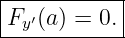
free, the variation is arbitrary and the coefficient of that variation must vanish. This is the source
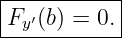
of the natural boundary condition
When an endpoint cost is present, the same reasoning modifies the natural condition rather than
replacing it. When the endpoint abscissa itself moves, the full transversality boundary form must
be used. These constructions are standard in the classical calculus of variations and in analytical
mechanics [1, 2, 3, 4].
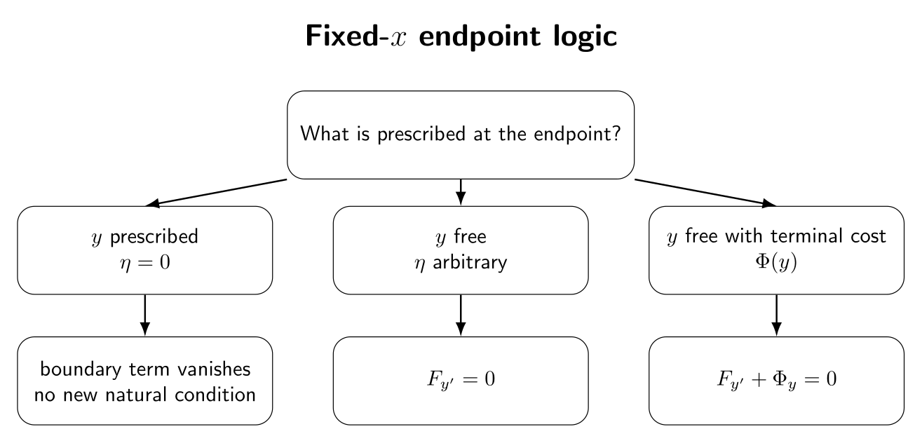
Figure. A compact decision map for fixed-x endpoint data. Prescribed endpoint values
eliminate the endpoint variation; free endpoint values produce a natural condition; an
explicit terminal cost contributes its own endpoint derivative.
1 How to use this set
Attempt every exercise before reading the solutions. For each problem use the same
sequence:
- identify what is fixed and what is free at each endpoint;
- write the admissible variation conditions;
- derive the Euler–Lagrange equation in the interior;
- retain the boundary term instead of discarding it automatically;
- impose the natural or transversality condition implied by the endpoint freedom;
- only then solve for the integration constants; and
- distinguish stationarity from any stronger minimum claim.
2 Exercises
Exercise 1: classify the endpoint data
For
assume the independent-variable endpoints a and b are fixed. For each case below, state the
endpoint conditions on the variation η and the resulting natural boundary condition, if
any.
- y(a) and y(b) are both prescribed.
- y(a) is prescribed and y(b) is free.
- y(a) is free and y(b) is prescribed.
- both y(a) and y(b) are free.
Explain why a free endpoint does not mean “there is no boundary condition.”
Exercise 2: the simplest one-free-end problem
Let
with
while y(L) is free.
- Derive the Euler–Lagrange equation.
- Derive the natural boundary condition at x = L.
- Solve for the stationary function.
- Prove directly that the stationary function is the global minimizer.
Exercise 3: a uniformly forced strip with a free right end
Consider
with
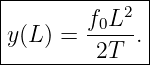
and y(L) free.
- Derive the interior Euler–Lagrange equation.
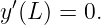
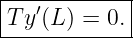
- Derive the natural condition at x = L.
- Solve for y(x).
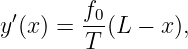
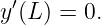
- Find y(L) and verify that the terminal slope is zero.
- Interpret Ty′ as the generalized boundary traction associated with the slope variable.
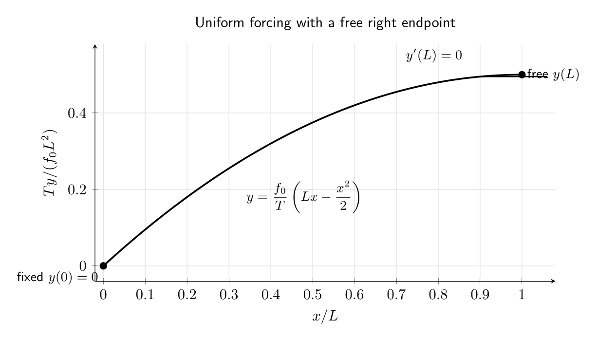
Figure. A constant distributed load with the left value fixed and the right value free. The
natural condition forces a horizontal tangent at the free endpoint.
Exercise 4: a terminal spring and a Robin-type condition
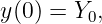
Let
with y(0) = 0 and y(L) free.
- Compute the first variation, including the variation of the terminal spring energy.
- Derive the interior equation.
- Show that the terminal condition is
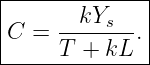
- Solve the complete boundary-value problem.
- Examine the limits k → 0 and k →∞ and interpret both.
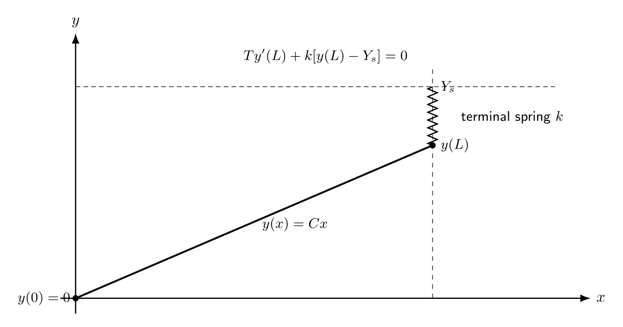
Figure. A free terminal value can be coupled to an endpoint energy. The resulting
boundary condition balances the interior conjugate quantity Ty′(L) against the spring
force generated by the terminal penalty.
Exercise 5: a prescribed endpoint load
Consider
with y(0) = 0 and y(L) free.
- Derive the natural terminal condition.
- Solve for y(x).
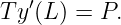
- Show that the boundary condition can be written
- Explain why the free-end condition is not y′(L) = 0 in this problem.
Exercise 6: both endpoint values free
Let
and suppose both y(0) and y(L) are free.
- Derive the Euler–Lagrange equation.
- Derive both natural boundary conditions.
- Solve the resulting boundary-value problem.
- Prove directly that the stationary solution is the unique global minimizer.
Exercise 7: free terminal position in mechanics
A particle moves vertically in a uniform gravitational field. Consider the action
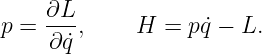
where tf is fixed, q(0) = q0 is prescribed, and q(tf) is free.
- Derive the equation of motion.
- Derive the natural condition at t = tf.
- Solve the trajectory completely.
- Explain the physical meaning of the natural condition in terms of canonical momentum.
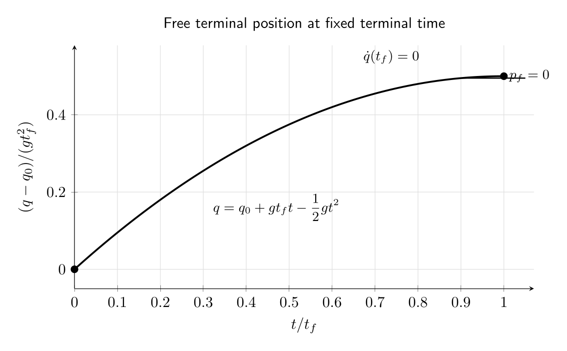
Figure. With terminal time fixed but terminal position free, stationarity requires the
canonical momentum at the final time to vanish. For the constant-gravity example this
means the trajectory reaches its turning point at tf.
Exercise 8: a conceptual free-terminal-time calculation
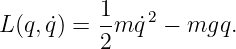
For a mechanical action
suppose the initial endpoint is fixed while the terminal point may move. CV05 showed that the
terminal boundary form can be written
where
- If tf is fixed and qf is free, what terminal condition follows?
- If qf is fixed and tf is free, what terminal condition follows?
- If both qf and tf are free independently, what two conditions follow?
- Explain why these are necessary stationarity conditions rather than minimum tests.
The appearance of p and H in the endpoint variation is the classical mechanics form of
transversality and is closely related to terminal conditions in optimal control [4, 5, 6].
3 Complete worked solutions
Solution 1: classify the endpoint data
For fixed a and b, integration by parts gives
On a stationary curve the interior Euler–Lagrange expression vanishes, so the endpoint logic is
controlled entirely by
(a) Both endpoint values prescribed.
Hence the boundary term vanishes automatically. There are no additional natural conditions.
(b) Left value prescribed, right value free.
Therefore
(c) Left value free, right value prescribed.
so
(d) Both values free.
Both endpoint variations are independent and arbitrary, so
The key conceptual point is that freedom makes the endpoint variation arbitrary. An arbitrary
variation is more restrictive on the coefficient, not less restrictive. Thus a free endpoint usually
creates a natural boundary condition.
Solution 2: the simplest one-free-end problem
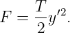
The integrand is
Hence
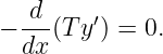
The Euler–Lagrange equation is
Since T is constant,
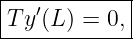
At the free endpoint x = L,
or simply
The general solution is
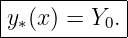
The natural condition gives C1 = 0, and y(0) = Y 0 gives C2 = Y 0. Therefore
To classify the solution, note that
For y∗ = Y 0, y∗′ = 0 and therefore
Thus
for every admissible y. The stationary function is therefore a global minimizer, not merely a
stationary candidate.
Solution 3: a uniformly forced strip with a free right end
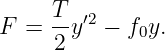
Here
Thus
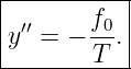
The Euler–Lagrange equation is
so
Because y(L) is free while L is fixed,
Integrating twice,
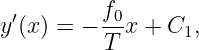
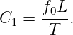
The fixed left endpoint gives C2 = 0. The free-end condition gives
hence
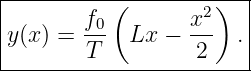
Therefore
At the free end,
Also
so indeed
The quantity Fy′ = Ty′ is the quantity conjugate to the endpoint value y. In this simple
one-dimensional elastic model it plays the role of a boundary traction. With no externally imposed
endpoint load, stationarity sets that traction to zero.
Solution 4: a terminal spring and a Robin-type condition
Write
with
The variation of the integral is
The terminal spring contributes
Because y(0) is fixed, η(0) = 0. Therefore
Interior stationarity gives
Since y(L) is free, η(L) is arbitrary, so
The interior solution is
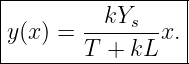
From y(0) = 0, D = 0. Hence y = Cx and the terminal condition becomes
Therefore
so
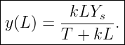
The stationary profile is
The endpoint value is
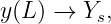
If k → 0, then C → 0 and the endpoint behaves like an unloaded free end. If k →∞,
then
so a very stiff terminal spring approaches a prescribed endpoint value. This is a useful bridge
between natural and essential boundary data.
Solution 5: a prescribed endpoint load
The integral part gives
The terminal load term contributes
Thus
The interior equation is
and the free terminal value gives
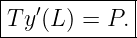
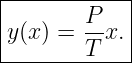
Since y = Cx + D and y(0) = 0, D = 0. The terminal condition gives
so
The free endpoint does not imply y′(L) = 0 because an external endpoint term is present. The
natural condition expresses a balance between the internal conjugate quantity Ty′ and the applied
terminal load P.
Solution 6: both endpoint values free
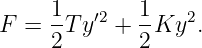
The integrand is
Therefore
The Euler–Lagrange equation is
or
Because both endpoint values are free,
The general solution is
Differentiate:
At x = 0,
so B = 0. Then
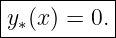
Since λ > 0 and L > 0, sinh(λL) > 0, hence A = 0. Therefore
Moreover,
with equality only if y′ = 0 and y = 0 throughout the interval. Thus y = 0 is the unique global
minimizer.
Solution 7: free terminal position in mechanics
Here the independent variable is time and
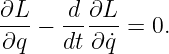
The Euler–Lagrange equation is
Since
we obtain
or
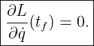
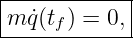
Because the terminal time tf is fixed but q(tf) is free, the natural condition is
Thus
or
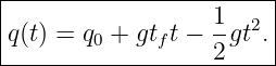
Integrating the equation of motion,
The natural condition gives
so
Integrating again,
The prescribed initial value gives C2 = q0. Therefore
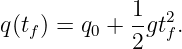
The final position is
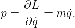
The canonical momentum is
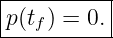
Thus a free terminal position at fixed terminal time requires
For this example, the stationary trajectory reaches its turning point exactly at the terminal
time.
Solution 8: a conceptual free-terminal-time calculation
The terminal boundary form is
(a) Fixed terminal time, free terminal position.
Here
while δqf is arbitrary. Therefore
(b) Fixed terminal position, free terminal time.
Here
while δtf is arbitrary. Therefore
(c) Both terminal position and terminal time free independently.
The variations δqf and δtf are independent, so both coefficients must vanish:
(d) Necessary versus sufficient.
These conditions come from requiring the first-order variation to vanish. They therefore identify
stationary candidates. They do not determine whether the candidate is a minimum, maximum, or
saddle. Classification requires additional information such as convexity or second-variation
tests.
4 Common mistakes
- Mistake: setting η = 0 at every endpoint automatically. This silently converts a
free-endpoint problem back into a fixed-endpoint one.
- Mistake: imposing Fy′ = 0 at an endpoint whose value is prescribed. The variation
already vanishes there, so no new natural condition follows.
- Mistake: assuming every free endpoint gives y′ = 0. The actual condition is Fy′ = 0,
or a modified balance when endpoint costs or loads are present.
- Mistake: forgetting the variation of an endpoint energy such as Φ(y(L)).
- Mistake: treating the natural condition as a replacement for the Euler–Lagrange
equation. A stationary solution normally must satisfy both the interior equation and
the relevant endpoint condition.
- Mistake: concluding “minimum” solely from Euler–Lagrange and natural boundary
conditions. They are first-order necessary conditions.
5 Summary of skills practiced
After completing this set, the reader should be able to
- translate endpoint freedom into conditions on the variation η;
- derive natural boundary conditions from the retained integration-by-parts term;
- solve one-free-end and two-free-end boundary-value problems;
- include endpoint loads and terminal spring energies consistently;
- recognize Robin-type conditions as variational boundary balances;
- interpret Fy′ as an endpoint-conjugate quantity such as traction or canonical
momentum;
- apply the fixed-terminal-time free-position condition pf = 0 in mechanics;
- interpret the free-terminal-time condition Hf = 0 when the final coordinate is fixed;
and
- keep stationarity separate from minimum classification.
CV05E2 will use the same endpoint boundary form when the terminal point is not fully free but
constrained to lie on a prescribed curve. That restriction couples the allowed endpoint variations
and produces the classical transversality relation.
References
References
[1] I. M. Gelfand and S. V. Fomin, Calculus of Variations, Dover Publications, 2000.
[2] Bruce van Brunt, The Calculus of Variations, Springer, 2004.
[3] Charles Fox, An Introduction to the Calculus of Variations, Dover Publications, 1987.
[4] Herbert Goldstein, Charles Poole, and John Safko, Classical Mechanics, 3rd ed.,
Addison Wesley, 2002.
[5] L. D. Landau and E. M. Lifshitz, Mechanics, 3rd ed., Course of Theoretical Physics,
Vol. 1, Pergamon Press, 1976.
[6] Donald E. Kirk, Optimal Control Theory: An Introduction, Prentice-Hall, 1970.

![[parent]](https://images.physicslibrary.org/images/uparrow.png)
![δJ = [F ′η]b .
boundary y a](https://images.physicslibrary.org/cache/objects/1201/make4ht/CalculusOfVariationsFreeEndpointProblemsAndWorkedSolutions0x.png)

![∫
b ′
J[y] = F (x,y,y )dx,
a](https://images.physicslibrary.org/cache/objects/1201/make4ht/CalculusOfVariationsFreeEndpointProblemsAndWorkedSolutions2x.png)
![∫
T- L ′ 2
J[y] = 2 y (x) dx, T > 0,
0](https://images.physicslibrary.org/cache/objects/1201/make4ht/CalculusOfVariationsFreeEndpointProblemsAndWorkedSolutions3x.png)
![∫ L[ T ]
J[y] = --y′2 − f0y dx, T > 0, f0 > 0,
0 2](https://images.physicslibrary.org/cache/objects/1201/make4ht/CalculusOfVariationsFreeEndpointProblemsAndWorkedSolutions5x.png)

![∫
L T- ′2 k- 2
J[y] = 2 y dx + 2 [y (L ) − Ys] , T > 0, k > 0,
0](https://images.physicslibrary.org/cache/objects/1201/make4ht/CalculusOfVariationsFreeEndpointProblemsAndWorkedSolutions7x.png)
![T y′(L) + k[y(L ) − Ys] = 0.](https://images.physicslibrary.org/cache/objects/1201/make4ht/CalculusOfVariationsFreeEndpointProblemsAndWorkedSolutions8x.png)
![∫ L
J [y] = T-y′2dx − P y(L), T > 0,
0 2](https://images.physicslibrary.org/cache/objects/1201/make4ht/CalculusOfVariationsFreeEndpointProblemsAndWorkedSolutions9x.png)
![∫
1- L[ ′2 2]
J[y] = 2 T y + Ky dx, T > 0, K > 0,
0](https://images.physicslibrary.org/cache/objects/1201/make4ht/CalculusOfVariationsFreeEndpointProblemsAndWorkedSolutions11x.png)
![∫ [ ]
tf 1- 2
S[q] = 2m ˙q − mgq dt,
0](https://images.physicslibrary.org/cache/objects/1201/make4ht/CalculusOfVariationsFreeEndpointProblemsAndWorkedSolutions12x.png)
![∫ tf
S [q] = L(q, ˙q,t)dt,
t0](https://images.physicslibrary.org/cache/objects/1201/make4ht/CalculusOfVariationsFreeEndpointProblemsAndWorkedSolutions13x.png)

![∫ b( d )
δJ = [Fy′η]ba + Fy − ---Fy′ ηdx.
a dx](https://images.physicslibrary.org/cache/objects/1201/make4ht/CalculusOfVariationsFreeEndpointProblemsAndWorkedSolutions16x.png)








![T ∫ L
J[y] = -- y′2dx ≥ 0.
2 0](https://images.physicslibrary.org/cache/objects/1201/make4ht/CalculusOfVariationsFreeEndpointProblemsAndWorkedSolutions32x.png)
![J[y∗] = 0.](https://images.physicslibrary.org/cache/objects/1201/make4ht/CalculusOfVariationsFreeEndpointProblemsAndWorkedSolutions33x.png)
![|------------|
-J[y] ≥-J[y∗]|](https://images.physicslibrary.org/cache/objects/1201/make4ht/CalculusOfVariationsFreeEndpointProblemsAndWorkedSolutions34x.png)




![∫ L ′
J[y] = F (y )dx + Φ (y(L)),
0](https://images.physicslibrary.org/cache/objects/1201/make4ht/CalculusOfVariationsFreeEndpointProblemsAndWorkedSolutions48x.png)
![T ′2 k 2
F = --y , Φ = -[y(L) − Ys] .
2 2](https://images.physicslibrary.org/cache/objects/1201/make4ht/CalculusOfVariationsFreeEndpointProblemsAndWorkedSolutions49x.png)
![∫ L
δJ = [T y′η]L − T y′′ηdx.
int 0 0](https://images.physicslibrary.org/cache/objects/1201/make4ht/CalculusOfVariationsFreeEndpointProblemsAndWorkedSolutions50x.png)
![δΦ = k[y(L) − Ys]η(L).](https://images.physicslibrary.org/cache/objects/1201/make4ht/CalculusOfVariationsFreeEndpointProblemsAndWorkedSolutions51x.png)
![∫
L ′′ ′
δJ = − Ty η dx + {T y (L) + k[y(L) − Ys]}η(L ).
0](https://images.physicslibrary.org/cache/objects/1201/make4ht/CalculusOfVariationsFreeEndpointProblemsAndWorkedSolutions52x.png)

![|--′-----------------------|
-Ty-(L)-+-k[y(L)-−-Ys] =-0.-](https://images.physicslibrary.org/cache/objects/1201/make4ht/CalculusOfVariationsFreeEndpointProblemsAndWorkedSolutions54x.png)



![∫ L
δJ = [T y′η]L − T y′′ηdx.
int 0 0](https://images.physicslibrary.org/cache/objects/1201/make4ht/CalculusOfVariationsFreeEndpointProblemsAndWorkedSolutions62x.png)
![δ[− P y(L)] = − Pη (L).](https://images.physicslibrary.org/cache/objects/1201/make4ht/CalculusOfVariationsFreeEndpointProblemsAndWorkedSolutions63x.png)
![∫
L ′′ ′
δJ = − T y η dx + [T y (L) − P] η(L).
0](https://images.physicslibrary.org/cache/objects/1201/make4ht/CalculusOfVariationsFreeEndpointProblemsAndWorkedSolutions64x.png)










![∫
1- L ( ′2 2)
J[y] = 2 Ty + Ky dx ≥ 0,
0](https://images.physicslibrary.org/cache/objects/1201/make4ht/CalculusOfVariationsFreeEndpointProblemsAndWorkedSolutions79x.png)