Calculus of Variations: Functional Evaluation and Comparison Exercises
This companion entry reinforces CV01 before any first-variation machinery is introduced. The
emphasis is deliberately elementary but fundamental: a functional assigns a scalar to an entire
admissible function, and the value of that scalar depends both on the formula for the functional
and on the function inserted into it.
The exercises develop four habits that are essential later in the course:
- identify the domain and admissible class before doing algebra;
- substitute a complete trial function into a functional carefully;
- compare several admissible candidates without assuming that stationarity machinery
is required; and
- recognize that a restricted family of functions can turn an infinite-dimensional problem
into an ordinary finite-dimensional one.

Figure. Evaluating a functional means selecting an admissible function, computing any
required derivatives, substituting the entire function into the functional, and reducing the
result to a scalar.
1 Exercises
Exercise 1: function or functional?
For each mapping below, determine whether it is an ordinary function, a functional, or can be
interpreted as either depending on its declared domain. For every functional, state a natural
domain on which it is well defined.
- f(x) = x2 + 1.
- J[y] = ∫
01y(x)2 dx.
- P[y] = y(1∕2).
- L[y] = ∫
01
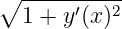 dx.
dx.
- M[y] = max 0≤x≤1|y(x)|.
Explain why a functional need not be written as an integral.
Exercise 2: evaluate one functional on several functions
Consider
Evaluate J[y] for each of the following functions:
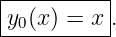
- y0(x) = 0,
- y1(x) = x,
- y2(x) = x2,
- y3(x) = sin(πx).
Rank the four functions by increasing functional value.
Exercise 3: the same formula, different variational problems
Consider the functional formula
Compare the following two admissible classes:
and
- Determine whether y = x, y = x2, and y = 0 belong to each class.
- Evaluate J on every candidate for which it is admissible.
- Explain why specifying only the formula for J does not completely specify the
variational problem.
- Without using Euler–Lagrange, identify the obvious global minimizer in 𝒜2 and justify
the claim.
Exercise 4: compare three admissible connecting curves
On the fixed-endpoint class
consider
and the three admissible curves
- Verify the endpoint conditions.
- Compute J[y1], J[y2], and J[y3] exactly.
- Which of these three trial curves has the smallest value?
- Does winning this three-curve comparison prove that the winning curve is the global
minimizer over all of 𝒜? Explain.
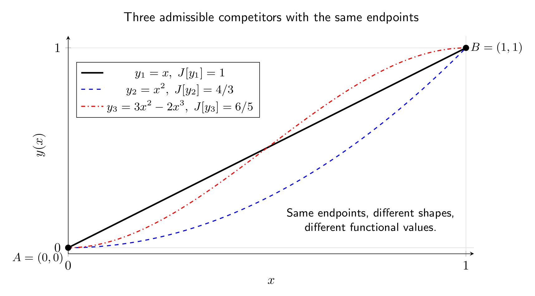
Figure. Three admissible competitors connecting the same endpoints. A functional can
rank these curves even before any variational derivative is introduced.
Exercise 5: arc length of a line and a parabola
For a graph y(x) on 0 ≤ x ≤ 1, define its length by
Both
connect (0, 0) to (1, 1).
- Compute L[y1] exactly.
- Show that
- Compare the two values numerically and interpret the result geometrically.
Exercise 6: restrict the problem to a one-parameter family
For
every member satisfies yc(0) = 0 and yc(1) = 1.
For the functional
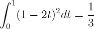
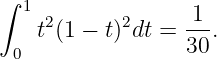
- compute the ordinary scalar function J(c) = J[yc];
- minimize J(c) using ordinary single-variable calculus;
- identify the corresponding curve;
- explain what has and has not been proved about the full admissible class.
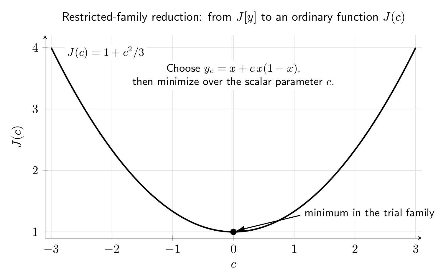
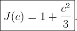
Figure. Restricting an infinite-dimensional search to the family yc = x + cx(1 − x)
produces the ordinary scalar function J(c) = 1 + c2∕3.
Exercise 7: a quadratic energy functional
Let
where T > 0 and K > 0 are constants. Evaluate E for the trial family
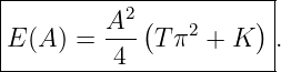
- Find E(A) exactly.
- Compare E[0], E[yA], and E[y2A].
- Explain why the quadratic dependence on amplitude is typical of small-deflection
elastic and field energies.
Exercise 8: evaluating a mechanical action on trial paths
Consider the one-dimensional action
with m > 0, k > 0, and fixed endpoint conditions q(0) = q(1) = 0. Restrict attention to the trial
family
- Compute S(a) = S[qa] exactly.
- For what relation between k and m is S(a) positive for every nonzero a in this trial
family? When is it negative?
- What happens when k = 10m?
- Explain why this example warns against assuming that an “action principle” always
means ordinary minimization of a positive quantity.
Exercise 9: an infimum that is not attained
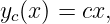
Let
and define
- Compute J[yc].
- Determine inf y∈𝒜J[y].
- Is that infimum attained by any admissible function?
- What change to the admissible set would make the infimum attained?
2 Solutions
Solution 1: function or functional?
(a) The mapping
is an ordinary real-valued function of a numerical variable x.
(b) The mapping
is a functional because its input is an entire function y. A natural domain is C0([0, 1]), although
much larger spaces such as L2(0, 1) are also possible.
(c) The map
is a functional if its input is a function y. A natural domain is C0([0, 1]). This example is important
because it is a functional that is not written as an integral.
(d) The arc-length map
is a functional. A classical domain is C1([0, 1]), possibly restricted by endpoint conditions.
(e) The map
is also a functional. For continuous functions on a compact interval the maximum exists, so
C0([0, 1]) is a natural domain.
Thus a functional is characterized by the nature of its input, not by whether its formula contains
an integral. Integrals are common because physical quantities such as length, action, energy, and
mass accumulate local contributions, but point evaluation and maximum norms are also
functionals.
Solution 2: evaluate one functional on several functions
The functional is
(a) For y0 = 0, both y0 and y0′ vanish, so
(b) For y1 = x, y1′ = 1, hence
(c) For y2 = x2, y
2′ = 2x, so
(d) For y3 = sin(πx),
Therefore
| J[y3] | = ∫
01![[ ]
sin2(πx ) + π2 cos2(πx)](https://images.physicslibrary.org/cache/objects/1198/make4ht/AdmissibleFunctionsExampleOfCalculusOfVariationsFunctionals29x.png) dx dx | (29)
|
| =  + +  = =  . . | (30) |
Numerically,
Thus the ranking is
from smallest to largest functional value.
Solution 3: the same formula, different variational problems
The functional formula is
(a) For 𝒜1, admissibility requires y(0) = 0 and y(1) = 1. Therefore
For 𝒜2, admissibility requires both endpoints to vanish. Hence
while y = x and y = x2 are not in 𝒜
2 because both equal 1 at x = 1.
(b) The admissible evaluations are
and
(c) The same integral expression can represent different optimization problems because the
competitors are different. The admissible class is part of the mathematical definition of the
problem.
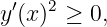
(d) Since
we have
for every admissible y. The function y = 0 belongs to 𝒜2 and attains J[0] = 0. Therefore it is a
global minimizer. In fact it is the unique global minimizer among C1 functions, because J[y] = 0
forces y′ = 0 everywhere, and the endpoint condition then forces y = 0.
Solution 4: compare three admissible connecting curves
(a) At x = 0,
At x = 1,
All three are admissible.
(b) For y1 = x,
For y2 = x2,
For
we have
Therefore
| J[y3] | = 36 ∫
01x2(1 − x)2 dx | (47)
|
| = 36 ∫
01(x2 − 2x3 + x4) dx | (48)
|
| = 36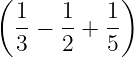 | (49)
|
| = 36 = =  . . | (50) |
Hence
(c) Among these three trial curves, the line y1 = x has the smallest value.
(d) No. This proves only that y1 beats the two specific competitors chosen here. The
full admissible class contains infinitely many other curves. A global-minimum proof
must compare against every admissible function or use a theorem that guarantees the
result.
CV01 itself gave such a direct proof by writing an arbitrary admissible curve as y = x + u with
u(0) = u(1) = 0, which yields
Solution 5: arc length of a line and a parabola
(a) For y1 = x, y1′ = 1, so
(b) For y2 = x2, y
2′ = 2x, hence
Use the standard antiderivative
Evaluating from 0 to 1 gives
Since
we obtain
(c) Numerically,
The straight segment is shorter. This agrees with Euclidean geometry: among all sufficiently
regular curves joining two fixed points in the plane, the straight line has the least length.
Solution 6: restrict the problem to a one-parameter family
The family is
Differentiate:
Then
| J(c) | = ∫
01![[1 + c(1 − 2x )]](https://images.physicslibrary.org/cache/objects/1198/make4ht/AdmissibleFunctionsExampleOfCalculusOfVariationsFunctionals63x.png) 2dx 2dx | (62)
|
| = ∫
01![[ ]
1 + 2c(1 − 2x) + c2(1 − 2x )2](https://images.physicslibrary.org/cache/objects/1198/make4ht/AdmissibleFunctionsExampleOfCalculusOfVariationsFunctionals64x.png) dx. dx. | (63) |
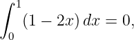
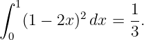
The linear term integrates to zero:
and
Therefore
(b) Ordinary calculus gives
Thus the unique minimum within this family occurs at
(c) The corresponding curve is
(d) We have proved that y = x minimizes J among the restricted one-parameter family yc. By
itself, this does not prove that it minimizes over the entire infinite-dimensional admissible class.
Restricted trial families are useful approximations, but the conclusion is only as broad as the
family searched.
This finite-dimensional reduction foreshadows the Ritz method developed much later in the
course.
Solution 7: a quadratic energy functional
For
we have
Substitute into the energy:
| E(A) | =  ∫
01 ∫
01![[ ]
T A2 π2cos2(πx ) + KA2 sin2(πx)](https://images.physicslibrary.org/cache/objects/1198/make4ht/AdmissibleFunctionsExampleOfCalculusOfVariationsFunctionals74x.png) dx dx | (72)
|
| =  A2 A2![[ (1 ) ( 1) ]
T π2 -- + K --
2 2](https://images.physicslibrary.org/cache/objects/1198/make4ht/AdmissibleFunctionsExampleOfCalculusOfVariationsFunctionals76x.png) . . | (73) |
Hence
Therefore
and
The factor-of-four scaling follows because both terms in the functional are quadratic in y or its
derivative. Linear elasticity, small oscillations, and many linear field theories produce quadratic
energies for exactly this reason.
Solution 8: evaluating a mechanical action on trial paths
The trial path is
so
Substitute into the action:
The needed integrals are
and
Therefore
| S(a) | =  − − | (83)
|
| =  (10m − k) . (10m − k) . | (84) |
(b) For every nonzero a, the sign is controlled by 10m − k:
while
(c) If k = 10m, then
for every amplitude a in this particular trial family.
(d) Mechanical action contains kinetic energy minus potential energy, not a manifestly positive
sum. Stationary-action principles therefore need not be ordinary global minimization statements.
Later entries will distinguish stationarity from minimum, maximum, and saddle behavior
rigorously.
Solution 9: an infimum that is not attained
For
we have
Because c > 0 can be chosen arbitrarily small,
However, no admissible c > 0 gives J[yc] = 0. The only parameter that would attain zero is
c = 0, and it is excluded from the admissible set. Thus the infimum exists but is not
attained.
If the admissible set is changed to
then c = 0 becomes admissible and the minimum is attained by y = 0.
This simple finite-dimensional example already captures an issue that becomes central in the direct
method of the calculus of variations: an infimum and an actual minimizer are different
mathematical statements.
3 Summary
These exercises reinforce the basic viewpoint of CV01. A functional is a map from functions to
scalars, and its optimization problem is defined not merely by its formula but also by its admissible
class. Direct substitution can rank trial curves, sometimes prove a global minimum from
positivity, and reveal important physical structure before any variational derivative is
introduced.
The restricted-family exercises also anticipate a recurring strategy:
In CV02 that scalarization is performed infinitesimally with y𝜖 = y + 𝜖η. In later numerical work it
becomes the foundation of Ritz and finite-dimensional approximation methods.

![[parent]](https://images.physicslibrary.org/images/uparrow.png)
![∫ 1
J[y] = (y (x )2 + y′(x)2)dx.
0](https://images.physicslibrary.org/cache/objects/1198/make4ht/AdmissibleFunctionsExampleOfCalculusOfVariationsFunctionals1x.png)
![∫ 1
J[y] = y′(x)2dx.
0](https://images.physicslibrary.org/cache/objects/1198/make4ht/AdmissibleFunctionsExampleOfCalculusOfVariationsFunctionals2x.png)
![𝒜 = {y ∈ C1([0,1]) : y(0) = 0, y(1) = 1} ,
1](https://images.physicslibrary.org/cache/objects/1198/make4ht/AdmissibleFunctionsExampleOfCalculusOfVariationsFunctionals3x.png)
![{ }
𝒜2 = y ∈ C1([0,1]) : y(0) = 0, y(1) = 0 .](https://images.physicslibrary.org/cache/objects/1198/make4ht/AdmissibleFunctionsExampleOfCalculusOfVariationsFunctionals4x.png)
![{ }
𝒜 = y ∈ C1 ([0,1]) : y(0) = 0, y(1) = 1 ,](https://images.physicslibrary.org/cache/objects/1198/make4ht/AdmissibleFunctionsExampleOfCalculusOfVariationsFunctionals5x.png)
![∫
1 ′ 2
J [y] = y(x) dx
0](https://images.physicslibrary.org/cache/objects/1198/make4ht/AdmissibleFunctionsExampleOfCalculusOfVariationsFunctionals6x.png)

![∫
1∘ -----′--2-
L[y] = 1 + y (x) dx.
0](https://images.physicslibrary.org/cache/objects/1198/make4ht/AdmissibleFunctionsExampleOfCalculusOfVariationsFunctionals8x.png)

![√ -- √ --
5 1 5 1 √ --
L [y2] = ----+ --arsinh(2) = ----+ --ln(2 + 5).
2 4 2 4](https://images.physicslibrary.org/cache/objects/1198/make4ht/AdmissibleFunctionsExampleOfCalculusOfVariationsFunctionals10x.png)

![∫
1 ′ 2
J[y] = y (x) dx,
0](https://images.physicslibrary.org/cache/objects/1198/make4ht/AdmissibleFunctionsExampleOfCalculusOfVariationsFunctionals12x.png)
![1 ∫ 1( )
E[y] = -- T y′(x)2 + K y(x)2 dx,
2 0](https://images.physicslibrary.org/cache/objects/1198/make4ht/AdmissibleFunctionsExampleOfCalculusOfVariationsFunctionals13x.png)

![∫ [ ]
1 1 2 1 2
S[q] = --m ˙q(t) − --kq(t) dt,
0 2 2](https://images.physicslibrary.org/cache/objects/1198/make4ht/AdmissibleFunctionsExampleOfCalculusOfVariationsFunctionals15x.png)


![∫ 1
J [y] = y(x)2dx.
0](https://images.physicslibrary.org/cache/objects/1198/make4ht/AdmissibleFunctionsExampleOfCalculusOfVariationsFunctionals18x.png)

![∫
1 2
J [y] = y(x) dx
0](https://images.physicslibrary.org/cache/objects/1198/make4ht/AdmissibleFunctionsExampleOfCalculusOfVariationsFunctionals20x.png)
![P [y] = y(1∕2)](https://images.physicslibrary.org/cache/objects/1198/make4ht/AdmissibleFunctionsExampleOfCalculusOfVariationsFunctionals21x.png)
![∫ 1∘ -------
L[y] = 1 + y′2dx
0](https://images.physicslibrary.org/cache/objects/1198/make4ht/AdmissibleFunctionsExampleOfCalculusOfVariationsFunctionals22x.png)
![M [y] = max |y(x)|
0≤x≤1](https://images.physicslibrary.org/cache/objects/1198/make4ht/AdmissibleFunctionsExampleOfCalculusOfVariationsFunctionals23x.png)
![∫
1 2 ′2
J [y ] = (y + y )dx.
0](https://images.physicslibrary.org/cache/objects/1198/make4ht/AdmissibleFunctionsExampleOfCalculusOfVariationsFunctionals24x.png)
![J[y0] = 0.](https://images.physicslibrary.org/cache/objects/1198/make4ht/AdmissibleFunctionsExampleOfCalculusOfVariationsFunctionals25x.png)
![∫ 1
J[y1] = (x2 + 1)dx = 1-+ 1 = 4-.
0 3 3](https://images.physicslibrary.org/cache/objects/1198/make4ht/AdmissibleFunctionsExampleOfCalculusOfVariationsFunctionals26x.png)
![∫
1 4 2 1 4 23
J [y2] = (x + 4x )dx = --+ --= --.
0 5 3 15](https://images.physicslibrary.org/cache/objects/1198/make4ht/AdmissibleFunctionsExampleOfCalculusOfVariationsFunctionals27x.png)



![∫ 1
J [y ] = y′2 dx.
0](https://images.physicslibrary.org/cache/objects/1198/make4ht/AdmissibleFunctionsExampleOfCalculusOfVariationsFunctionals35x.png)


![∫
1
J[x] = 1dx = 1,
0](https://images.physicslibrary.org/cache/objects/1198/make4ht/AdmissibleFunctionsExampleOfCalculusOfVariationsFunctionals38x.png)
![∫ 1 4
J[x2] = (2x )2dx = -,
0 3](https://images.physicslibrary.org/cache/objects/1198/make4ht/AdmissibleFunctionsExampleOfCalculusOfVariationsFunctionals39x.png)
![J [0 ] = 0.](https://images.physicslibrary.org/cache/objects/1198/make4ht/AdmissibleFunctionsExampleOfCalculusOfVariationsFunctionals40x.png)
![J[y] ≥ 0](https://images.physicslibrary.org/cache/objects/1198/make4ht/AdmissibleFunctionsExampleOfCalculusOfVariationsFunctionals42x.png)


![J[y1] = 1.](https://images.physicslibrary.org/cache/objects/1198/make4ht/AdmissibleFunctionsExampleOfCalculusOfVariationsFunctionals45x.png)
![∫ 1 4
J [y2] = 4x2dx = -.
0 3](https://images.physicslibrary.org/cache/objects/1198/make4ht/AdmissibleFunctionsExampleOfCalculusOfVariationsFunctionals46x.png)


![|----------------------------------|
| 6 4 |
|J[y1] = 1 < J [y3] =-< J[y2] = --.
--------------------5------------3-](https://images.physicslibrary.org/cache/objects/1198/make4ht/AdmissibleFunctionsExampleOfCalculusOfVariationsFunctionals52x.png)
![∫ 1 ′2
J [y ] = 1 + u dx ≥ 1.
0](https://images.physicslibrary.org/cache/objects/1198/make4ht/AdmissibleFunctionsExampleOfCalculusOfVariationsFunctionals53x.png)
![∫ |---|
1√ -- |√ -|
L [y1] = 2 dx = ---2-.
0](https://images.physicslibrary.org/cache/objects/1198/make4ht/AdmissibleFunctionsExampleOfCalculusOfVariationsFunctionals54x.png)
![∫ 1√ --------
L[y2] = 1 + 4x2dx.
0](https://images.physicslibrary.org/cache/objects/1198/make4ht/AdmissibleFunctionsExampleOfCalculusOfVariationsFunctionals55x.png)

![√ --
--5- 1-
L[y2] = 2 + 4 arsinh (2).](https://images.physicslibrary.org/cache/objects/1198/make4ht/AdmissibleFunctionsExampleOfCalculusOfVariationsFunctionals57x.png)

![|--------√------------------|
| 5 1 √ --|
|L [y2] = ----+ --ln(2 + 5).
----------2----4------------](https://images.physicslibrary.org/cache/objects/1198/make4ht/AdmissibleFunctionsExampleOfCalculusOfVariationsFunctionals59x.png)
![L [y1] ≈ 1.41421, L [y2] ≈ 1.47894.](https://images.physicslibrary.org/cache/objects/1198/make4ht/AdmissibleFunctionsExampleOfCalculusOfVariationsFunctionals60x.png)






![E [0] = 0,](https://images.physicslibrary.org/cache/objects/1198/make4ht/AdmissibleFunctionsExampleOfCalculusOfVariationsFunctionals78x.png)
![A2- 2
E [yA] = 4 (Tπ + K ),](https://images.physicslibrary.org/cache/objects/1198/make4ht/AdmissibleFunctionsExampleOfCalculusOfVariationsFunctionals79x.png)
![E [y2A] = 4E [yA ].](https://images.physicslibrary.org/cache/objects/1198/make4ht/AdmissibleFunctionsExampleOfCalculusOfVariationsFunctionals80x.png)






![∫ |---|
1 2 2 |c2 |
J[yc] = c x dx = |-- .
0 -3--](https://images.physicslibrary.org/cache/objects/1198/make4ht/AdmissibleFunctionsExampleOfCalculusOfVariationsFunctionals93x.png)
![|------------|
|inf J [y] = 0 .
y∈𝒜----------|](https://images.physicslibrary.org/cache/objects/1198/make4ht/AdmissibleFunctionsExampleOfCalculusOfVariationsFunctionals94x.png)

![choose a parameterized family of functions =⇒ reduce J [y] to an ordinary function of parameters.](https://images.physicslibrary.org/cache/objects/1198/make4ht/AdmissibleFunctionsExampleOfCalculusOfVariationsFunctionals96x.png)