A Geometrical Theory of Diffraction
Joseph B. Keller
1. Introduction
Geometrical optics is a theory of Light propagation based on the assumption that light travels
along certain curves, called rays, which are determined by the laws of geometrical optics. Although
experience has shown that this theory is essentially correct, there are still many cases in which
light appears in places where there are no rays (i.e., in shadows). Such discrepancies between
experience and geometrical optics are called diffraction effects. It is the purpose of this article to
show that geometrical optics can be so modified as to include diffraction. The modification consists
in introducing new rays, called diffracted rays, by extending the laws of geometrical optics. These
new rays account for the appearance of light in shadows and also alter the light in lit
regions.
It seems evident that diffracted rays should be produced when a ray hits an edge or a vertex or
when a ray grazes an interface or a boundary. Geometrical optics does not describe what happens
in any of these cases; hence we will extend it to do so. Then it will yield the diffracted
rays.
Our extension of the laws of optics will be presented in two equivalent forms. The first is the
explicit form, in which we enumerate the different situations in which diffracted rays
are produced and describe the different kinds of diffracted rays which occur in each
case. The second formulation is based upon an extension of Fermat’s principle. The
equivalence of the two formulations follows from the usual considerations of the calculus of
variations.
Once the diffracted rays have been introduced, we shall define diffracted wavefronts and the phase,
or eiconal, function by means of them. In this way we shall obtain new solutions of the eiconal
equation. Conversely, from appropriate solutions of this equation, diffracted wavefronts and rays
can be determined.
A number of examples in which diffracted rays occur will be described to illustrate this part of our
theory. In these examples the diffracted rays cover the shadows of ordinary geometrical optics.
However, we shall also find certain cases in which shadows remain even after the introduction of
diffracted rays. To obtain rays in such shadow regions, we shall further extend the concept of a ray
by introducing imaginary rays. These rays can be used in much the same way as real rays. For
example, a complex phase function can be defined in terms of them. It provides the
analytic continuation, from a lit region into the shadow, of a solution of the eiconal
equation.
The second part of our theory shows how the rays and wavefronts can be used for the quantitative
description of the light distribution. This necessitates the introduction of an amplitude function
and certain principles for its determination.
Finally we shall discuss the relation of our theory to previous work on diffraction. This may
partially justify the introduction of the new rays by showing how some kinds of them have already
appeared in special cases.
All our considerations can be applied to other single-integral variational problems and to other
first-order partial differential equations in any number of variables. They lead to the introduction
of diffracted extremals and diffracted characteristics and of complex characteristics. With the aid
of these characteristics, additional branches of solutions of first-order equations can be constructed.
Complex solutions, which are analytic continuations of certain real solutions, can also be obtained
for analytic equations.
As an example, consider the Hamilton-Jacobi equation of Classical Mechanics. The characteristics
of this equation are the classical-mechanical trajectories which satisfy Hamilton’s canonical
equations or Newton’s equations of motion. The complex characteristics are complex-valued
solutions of Newton’s or Hamilton’s equations. These complex trajectories enter the “forbidden
regions” into which real trajectories cannot penetrate. They enable us to continue solutions of the
Hamilton-Jacobi equation into these regions, and yield complex values for the solutions there. The
appearance of trajectories in forbidden regions is related to the “tunnel effect” of quantum
mechanics. In fact, the present considerations provide a new classical interpretation of this
effect.
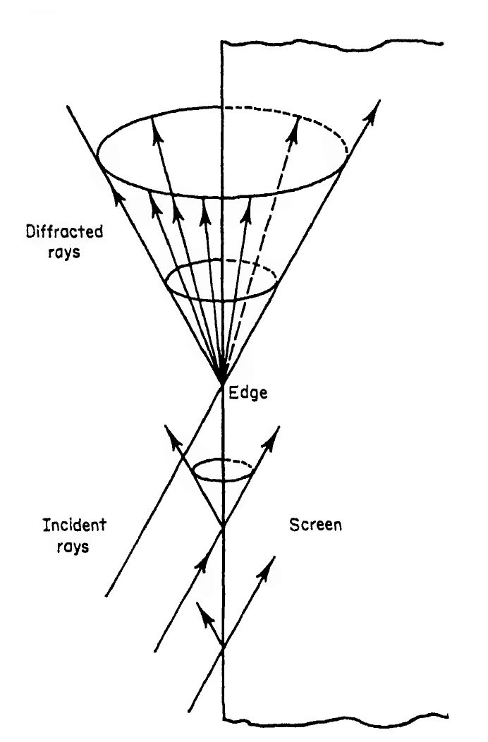
Fig. 1. The cone of diffracted rays produced by an incident ray which hits the edge of a thin
screen.
2. Diffracted rays
The first kind of diffracted ray is produced when an incident ray hits an edge (see Figs. 1 to 4).
The incident ray produces infinitely many diffracted rays, traveling in directions determined by the
law of diffraction. This law states that each diffracted ray which lies in the same medium as the
incident ray makes the same angle with the edge as does the incident ray. Furthermore, the
incident and diffracted rays lie on opposite sides of the plane normal to the edge at the point of
diffraction. However, the diffracted ray need not lie in the same plane as the incident ray and the
edge. Therefore the diffracted rays form the surface of a cone with its vertex at the point of
diffraction.
If a diffracted ray and the incident ray lie in different media, the angle between the diffracted ray
and the edge is related to the angle between the incident ray and the edge by Snell’s law (see Fig.
5a). But here again, the diffracted ray is not restricted to lie in the same plane as the
incident ray and the edge. Therefore these diffracted rays also form the surface of a
cone.
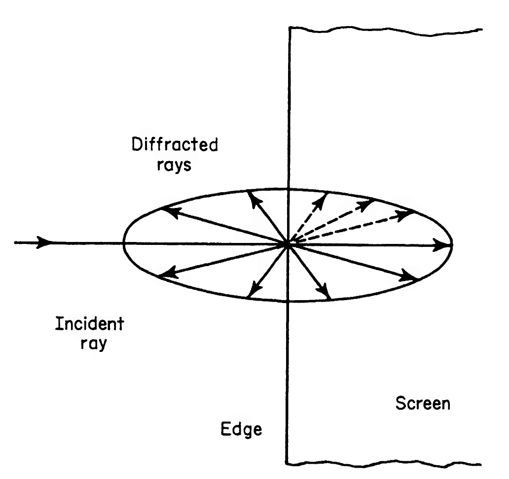
Fig. 2. The plane of diffracted rays produced by a ray normally incident on the edge of a thin
screen.
When an incident ray hits a vertex (e.g., a junction of two or more edges), it produces infinitely
many diffracted rays which leave the vertex in all directions (see Fig. 6). Thus at a vertex a single
incident ray produces a two-parameter family of diffracted rays.
When a ray grazes an interface or boundary surface (i.e., when it is tangent to the
surface), the ray splits in two (see Fig. 7). One part continues, unaffected by the surface, as
an ordinary ray. The other part travels along the surface. Its path on the surface is a
surface ray, i.e., a curve which satisfies the differential equations for a ray, when these
equations are specialized to a surface. A surface ray also makes Fermat’s integral stationary
among all curves lying on the surface. At every point on its path this ray again splits
in two, one part continuing along the surface and the other part leaving the surface
along the tangent to the surface ray, provided that the tangent lies on the same side of
the surface as the surface ray. In defining a surface ray, one must use the value of the
index of refraction appropriate to that side of the surface from which the incident ray
comes.
If the surface ray lies on that side of the surface having the lesser index of refraction, it also sheds
another diffracted ray at each point on its path (see Fig. 8). This diffracted ray is a critically
refracted ray, which leaves the surface at the critical angle on the side opposite the surface ray.
Conversely, a surface ray is produced when a ray is incident at the critical angle on that side of the
surface having the greater index of refraction (see Fig. 9). In this case the refracted ray is initially
tangent to the surface and then proceeds along it as a surface ray. Surface rays are
also produced by a ray incident at an edge or a vertex, since in these cases some of
the diffracted rays leave the edge or vertex along the surfaces meeting there (see Fig.
5).
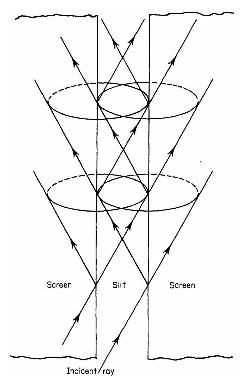
Fig. 3. The diffracted rays produced by a plane wave obliquely incident upon a slit in a thin
screen. The two incident rays which hit the slit edges are shown, along with some of the singly
diffracted rays which they produce. One diffracted ray from each edge is shown crossing the slit
and hitting the opposite edge, producing doubly diffracted rays and then triply diffracted rays.
When a ray is incident on a surface of discontinuity of any derivative of the index of refraction, it is
reflected and refracted just as at a surface of discontinuity of the index itself. Similarly, diffracted
rays are produced when incident rays hit edges or vertices of such surfaces or when they graze
these surfaces. In other words, such surfaces behave in all respects like discontinuity surfaces of the
index of refraction itself.
Just as discontinuity surfaces of derivatives of the index of refraction must be included as surfaces,
so must lines of discontinuity of any derivatives of surfaces be counted as edges. Thus an
ordinary edge is a line along which first derivatives of a surface (i.e., the slopes) are
discontinuous. Similarly, a line along which second derivatives of a surface (i.e., the
curvatures) are discontinuous must also be counted as an edge. Discontinuities in higher
derivatives of a surface also yield edges. In the same way, discontinuities in any derivatives of
edges must be counted as vertices. In addition, isolated points (not on edges) at which
derivatives of a surface are discontinuous also play the role of vertices. The apex of a
cone is an example of such a point. Diffracted rays are produced when rays hit any of
these edges or vertices, in the same way as they are produced at ordinary edges and
vertices.
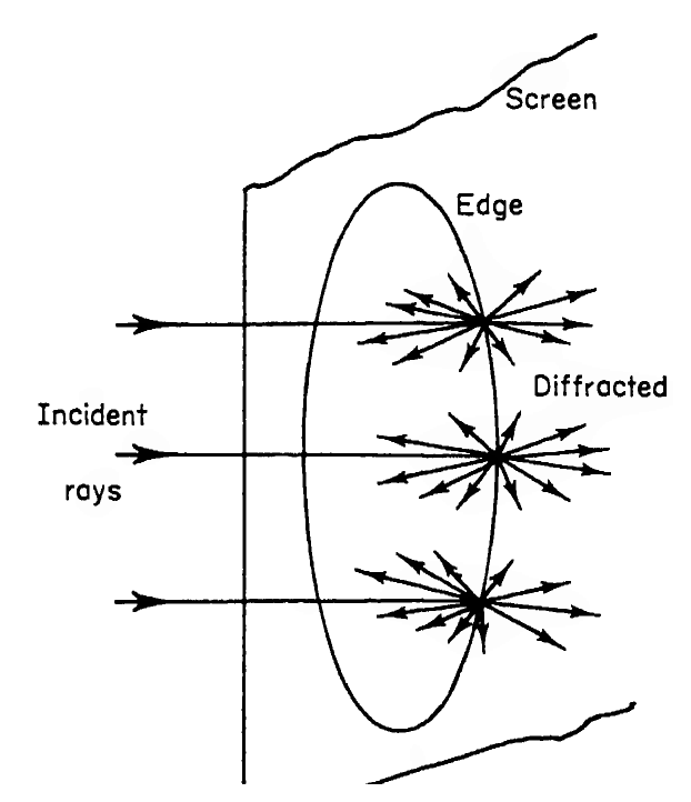
Fig. 4. A plane wave normally incident upon an aperture in a plane screen. The incident rays are
normal to the edge; hence the rays diffracted from each point of the edge lie in a plane normal to
the edge.
On the basis of the preceding descriptions, we may say that a ray is diffracted whenever it hits an
edge or vertex or grazes a surface. In every such case the ray produces infinitely many diffracted
rays. Thus the process of diffraction, which occurs in these cases, splits a single ray into infinitely
many diffracted rays. It is natural to expect that the light intensity associated with these diffracted
rays, as well as with rays reflected from discontinuity surfaces of derivatives of the refractive index,
is much smaller than that associated with the incident ray. This is indeed the case,
and is of particular importance in using our theory for the quantitative calculation of
intensities.
Away from discontinuity or boundary surfaces, all rays—both ordinary and diffracted—are
determined by the usual laws of geometrical optics. These laws, plus the laws of reflection and
refraction and the foregoing laws governing diffraction, completely determine all real
rays.
As a consequence of the theory of diffraction just described, diffracted rays will exist, in addition to
ordinary rays, in any medium which is bounded or in which the refractive index or any of its
derivatives is discontinuous. Of course, in specific examples the incident rays might be so arranged
that no diffraction occurs (see Fig. 10). In such examples no incident ray can hit an edge or graze a
surface; hence no shadows can be formed. Therefore the absence of diffracted rays in these
examples is not unexpected.
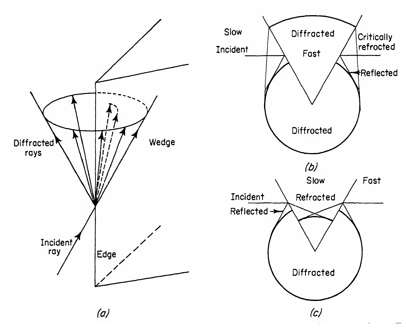
Fig. 5. (a) Some of the diffracted rays produced by a ray incident on the edge of a wedge. The
light velocity within the wedge is greater than it is outside the wedge. Therefore the angle
between the refracted rays and the edge is less than that between the incident ray and the edge.
(b) A section of the wavefront resulting from incidence of a plane wave upon a wedge. The
velocity within the wedge is greater than that outside. The incident, reflected, refracted, and
diffracted wavefronts are shown. The plane wavefronts produced by rays critically refracted into
the outer region from the diffracted wavefront inside the wedge are also shown. (c) A section of
the wavefront resulting from incidence of a plane wave on a wedge. The velocity within the wedge
is less than that outside. The incident, reflected, refracted, and diffracted wavefronts are shown.
3. Examples
Let us now consider some examples of diffracted rays. First, consider a plane wave (i.e., a set of
parallel rays) incident obliquely upon a thin opaque screen in the form of a half plane (see Fig. 1).
If the medium is homogeneous, then all the rays, incident, reflected, and diffracted, are straight
lines. The only diffracted rays are produced by those incident rays which hit the edge of the
screen. Since the incident rays are parallel to each other, the cones of diffracted rays
will also be parallel to each other. Each point of the edge will be the vertex of a cone.
One diffracted ray will reach each point in the medium, accounting for the appearance
of light in the “shadow” and also providing additional light rays in the illuminated
region.
If the incident rays are perpendicular to the edge instead of being oblique, the diffracted rays will
also be perpendicular to the edge (see Fig. 2). Thus in this case each cone of diffracted rays is
opened up to become a plane of diffracted rays.
As a third example, consider a plane wave incident obliquely upon a slit in a thin opaque screen
(see Fig. 3). The rays which hit the edges of the screen give rise to diffracted rays. Some of the rays
diffracted from one edge will hit the other edge and give rise to a new set of diffracted rays. Some
of these new rays will in turn hit the opposite edge, producing still other diffracted
rays, etc. Thus, in this case there is an infinite set of multiply diffracted rays. Some of
these rays are shown in Fig. 3. These singly and multiply diffracted rays are the only
diffracted rays which occur in this problem, and they account for the occurrence of light in
the shadow behind the screen. In addition, the usual incident and reflected rays are
present.
As a fourth example, let us consider a plane wave normally incident upon a plane screen which
contains an aperture with a smooth rim (see Fig. 4). Each incident ray which hits the rim is
perpendicular to it. Therefore each set of diffracted rays lies in the plane perpendicular to the edge
at the point of diffraction. As in the case of the slit, multiply diffracted rays will also be
produced. However, the cones of multiply diffracted rays will in general not be planes,
since the diffracted rays which produce them will in general not be perpendicular to the
edge.
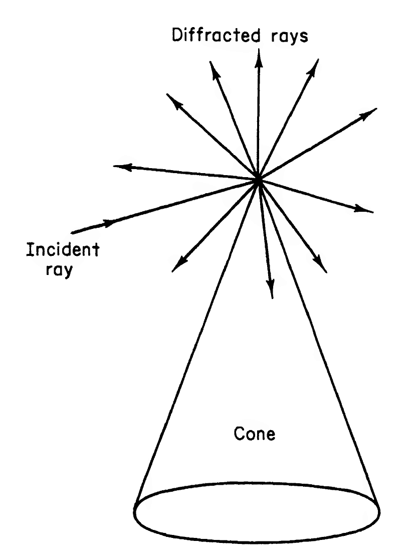
Fig. 6. Diffracted rays produced by a ray hitting the tip of an opaque cone. The diffracted rays
emanate from this tip in all directions.
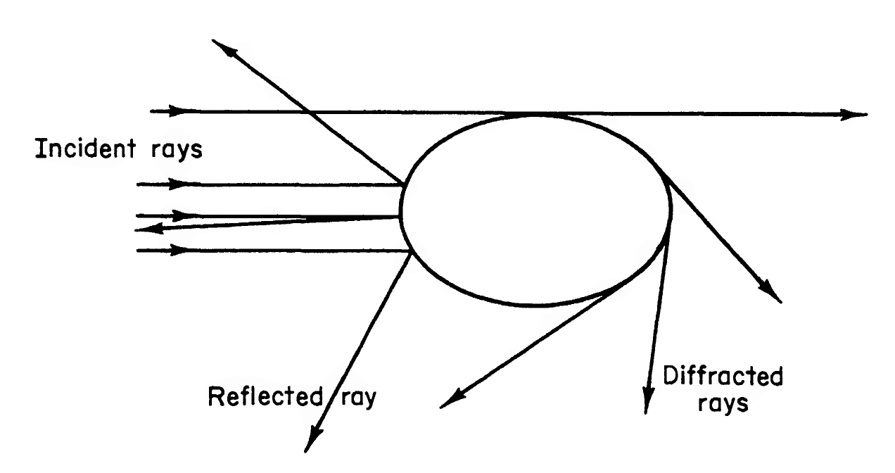
Fig. 7. Some of the diffracted and reflected rays produced when a plane wave hits an opaque
convex cylinder. One of the two grazing (tangent) rays is shown. This ray splits, part continuing
unaffected and part running along the cylinder surface. At each point of its path this surface ray
sheds a diffracted ray along the tangent to its path.
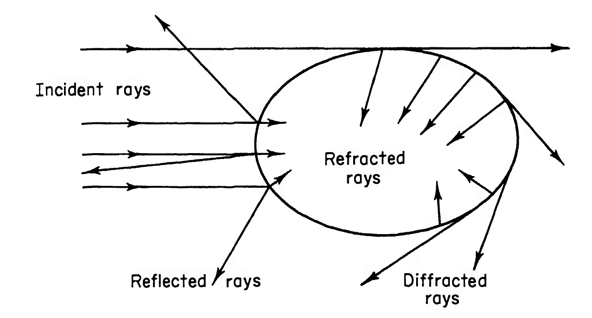
Fig. 8. Some of the diffracted, reflected, transmitted, and critically refracted rays produced when
a plane wave hits a convex cylinder of lower light velocity than the surrounding medium. One of
the two grazing rays is shown, along with some of the diffracted and critically refracted rays it
produces.
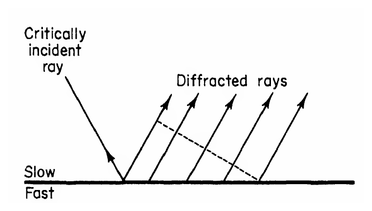
Fig. 9. A ray incident at the critical angle on a plane interface between two media. Some of the
resulting diffracted rays are shown. The dotted line is a section of the diffracted wavefront.
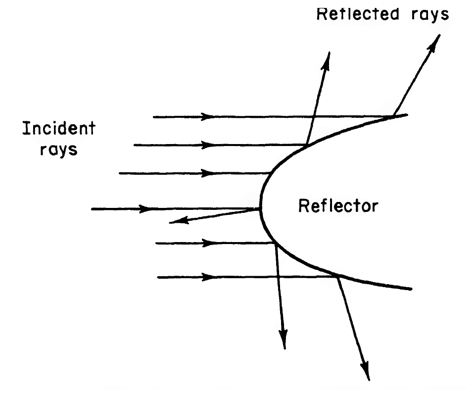
Fig. 10. A case in which no diffracted rays occur. No incident ray is tangent to the reflecting
surface.
In all the preceding examples, the diffracting edge is a caustic of the diffracted rays, i.e., a locus of
points of intersection of neighboring rays. Obviously, this is always the case with a diffracting edge.
However, in the last example above, the singly and multiply diffracted rays also possess other
caustics in addition to the edge. The caustic of the singly diffracted rays can be determined very
simply, because these rays lie in planes normal to the edge. Therefore, to locate the intersections of
neighboring rays, it suffices to consider the intersection of the neighboring planes which contain the
rays. Since all these planes are perpendicular to the plane of the screen, any two of
them must intersect in a straight line which is also perpendicular to the screen. As the
caustic is made up of such lines, it is a cylinder with generators perpendicular to the
screen.
To determine its cross section, we consider the curve of intersection of the cylinder and the plane of
the screen. In the plane of the screen, the diffracted rays are perpendicular to the rim, and
therefore their envelope is just the envelope of the normals to the rim. But this envelope is called
the evolute of the rim. Thus we see that the caustic of the singly diffracted rays is a
cylinder with generators normal to the screen and with the evolute of the rim as its cross
section.
If the screen is removed and replaced by a thin plate having the same rim as the aperture, the
preceding considerations apply equally well. This fact is a geometrical form of Babinet’s principle.
Furthermore, in the case of the plate, the caustic just described will lie (at least partly) in the
shadow of the plate. A cross section of it would appear as a bright line in the shadow, since light
intensity is greater at a caustic than elsewhere. If the plate has a circular rim, the evolute is a
single point, the center, and the caustic is just the axis of the circular plate. The resulting bright
spot on the axis is well known experimentally. The bright lines in the shadows of plates of other
shapes have also been observed and found to be the evolutes of the rims [2], as the above
considerations predict.
In the case of a plane wave obliquely incident upon a flat plate, a more detailed analysis shows that
the caustic of the singly diffracted rays approaches a cylindrical shape far behind the plate. The
generators of this limiting cylinder are parallel to the shadow boundary (i.e., to the incident-ray
direction). The cross section of this cylinder is the evolute of the cross section of the
shadow, i.e., of the curve obtained by cutting the shadow with a plane perpendicular to
the incident-ray direction. This shadow cross section is just a projection of the rim of
the plate. Thus, far behind a plate illuminated obliquely, there should be a bright line
in any cross section of the shadow, and it should be the evolute of the boundary of
the shadow. This prediction of the theory is also in agreement with the experimental
observations of the bright lines in the shadows of various plates illuminated obliquely [3].
If the bright lines had also been observed closer to the plates, they should have been
found to differ from the evolutes described above. However, such observations were not
made.
Let us now examine another example, in which a plane wave in a homogeneous medium is incident
upon a wedge of a different material. The incident rays corresponding to the plane wave will be
reflected and refracted at the surfaces of the wedge in the usual manner. In addition, the rays
which hit the edge will produce cones of diffracted rays, as in the preceding examples.
However, now some diffracted rays will also be produced inside the wedge (see Fig. 5a).
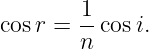
If i denotes the angle between an incident ray and the edge and r denotes the angle
between one of the resulting diffracted rays and the edge, then r is determined by the
equation
Here n is the relative refractive index of the two materials; i.e., n is the velocity in the surrounding
medium divided by the velocity in the wedge. Thus if the light velocity is faster within the wedge
material, the angle r is smaller than i.
Of the diffracted rays produced inside the wedge by a single incident ray, one proceeds along
each wall of the wedge. These two rays are surface rays within the faster medium, if
n < 1. Therefore they shed refracted rays back into the surrounding medium all along
their paths. These refracted rays leave the surface at the critical angle ic determined
by

They also lie in a plane normal to the surface. The “first” critically refracted ray coincides
with one of the diffracted rays produced by the incident ray in the outer medium, as
can be shown by simple trigonometry. Thus the shed refracted rays due to a single
incident ray lie in a plane sector bounded by the outer diffracted cone and a wall of
the wedge. The refracted rays shed from one wall of the wedge due to all the incident
rays are all parallel to each other and thus form a plane wave. In each medium the
cones of diffracted rays from the different points on the edge are also parallel to each
other and form a conical wave. Some sections of these wavefronts are shown in Fig.
5b and 5c. When n > 1, that is, when the faster medium is outside the wedge, the
refracted rays are shed into the wedge, and then the resulting plane waves lie inside the
wedge.
Next, suppose that a plane wave is incident upon an opaque cone, as in Fig. 6. Then, in
addition to the usual reflected rays, diffracted rays will be produced by that incident
ray which hits the vertex or tip of the cone. These rays will go in all directions from
the tip, and the corresponding diffracted wavefronts will be spheres with the tip as
center.
Let us now consider a plane wave normally incident upon an opaque cylinder of convex
cross section in a homogeneous medium (see Fig. 7). In this case, in addition to the
reflected rays, two surface rays will be produced by the two incident rays tangent to
the cylinder. These rays will lie in a plane normal to the axis of the cylinder and will
encircle the cylinder in opposite directions. At each point on its path each surface ray will
shed a diffracted ray along the tangent to the cross section of the cylinder (see Fig. 7).
Two diffracted rays will pass through each point in space, one coming from each of
the surface rays. The two rays through a given point are the two tangents to the cross
section which pass through that point. Actually, each of these rays represents an infinite
number of diffracted rays, one being shed by the surface ray each time it encircles the
cylinder. These rays account for the illumination in the shadow region and also provide
additional light in the lit region. The cross sections of the diffracted wavefronts, i.e., the
surfaces orthogonal to the diffracted rays, are just the involutes of the cross section of the
cylinder.
Suppose that the cylinder of the previous example is composed of a homogeneous material with a
lower light velocity and therefore a higher refractive index than the surrounding medium. Then the
incident rays which hit the cylinder will produce refracted rays inside the cylinder in addition to
the reflected rays in the surrounding medium (see Fig. 8). These refracted rays will hit the cylinder
surface and again produce reflected and transmitted rays, and this process will be repeated ad
infinitum. All of these multiply reflected and transmitted rays are ordinary rays. In
addition to them, the grazing rays will produce diffracted rays in the outer medium as
before. But now the surface rays will also shed refracted rays into the cylinder. These
refracted rays will leave the surface at the critical angle of refraction. Once inside the
cylinder, these diffracted rays will hit the opposite surface and be reflected and refracted,
etc.
As a final example, let us consider a spherical wave incident upon the plane interface
between two homogeneous media, as shown in Fig. 9. The corresponding incident rays
are straight lines emanating from the center of the spherical wave. They are reflected
and refracted at the interface in the usual way. However, if the second medium has the
faster light velocity, there is a critical angle at which the refracted ray is parallel to the
interface. Therefore this critically refracted ray is a surface ray in the faster medium.
Consequently, it sheds refracted rays back into the slower medium. These shed rays
leave the interface at the critical angle. The corresponding diffracted wavefronts are
cones, one of which is shown in cross section in Fig. 9. It appears there as a straight-line
segment.
4. A generalization of Fermat’s principle
In Sec. 2 we extended the laws of geometrical optics by introducing diffracted rays and giving an
explicit characterization of them. Now we shall consider an alternative (but equivalent) extension
of the laws of geometrical optics based upon a generalization of Fermat’s principle. This principle,
which is the basis of ordinary optics, involves the index of refraction n(x). This is a real
positive function which characterizes the optical behavior of the medium. In terms of
it the optical length L of any curve x(s) connecting two points P and Q is defined
as
The parameter s denotes arc length.
Fermat’s principle states that the optical rays connecting P and Q are those curves which make L
stationary in the class C0 of all smooth curves joining P and Q. This principle applies to an
unbounded continuous medium (i.e., one in which n is continuous). It does not apply to bounded
or discontinuous media [i.e., media in which n(x) is discontinuous]. We may try to apply it to such
media by considering, instead of C0, a class of curves with a finite number of corners. However this
formulation turns out to be unsatisfactory, because it yields only some rays, “direct” ones, but
does not include any reflected rays.
In order to obtain a principle valid for ordinary optics in discontinuous media, we introduce for
each integer r ≥ 0 the class of curves Cr. This is the class of curves with exactly r points on the
boundaries or discontinuity surfaces of the medium. These points are to be inner points of these
surfaces; i.e., they may not lie on edges or vertices. Now we formulate Fermat’s principle
as follows: The rays are those curves in each class Cr which make the optical length
stationary in Cr. Upon examining the consequences of this formulation, we find that the
class C0 yields rays which do not touch the boundary or discontinuity surfaces; C1
yields singly reflected or refracted rays; and Cr yields r-tuply reflected and/or refracted
rays.
The preceding formulation of Fermat’s principle for discontinuous and/or bounded media is
presumably implicit in older formulations of geometrical optics. Although it includes reflected rays,
it still fails to take account of diffracted rays. Therefore we shall further modify Fermat’s principle
by introducing additional classes of curves. For each triple of nonnegative integers r,s,t we shall
define the class Drst. This class consists of curves with r smooth arcs on the boundary or
discontinuity surfaces, s points on edges of the boundary or discontinuity surfaces, and t points
on vertices of these surfaces. Any number of the r arcs may be degenerate arcs, i.e.,
points. To each arc the value of n on one side of the surface is assigned. We now define
the rays as those curves in each class Drst which make the optical length stationary in
Drst.
The class D000 is the previously considered class C0, and thus it yields the direct rays. The
class Dr00 contains the previously considered class Cr and thus yields r-tuply reflected
and/or refracted rays. Each ray in any of the other classes has at least one point on
an edge or vertex and is thus a new ray not included in ordinary optics. Some of the
rays in Dr00 are also new rays, since they have arcs on the boundary or discontinuity
surfaces.
From the above extension of Fermat’s principle a number of conclusions can be drawn which suffice
to characterize the rays explicitly. First, let us consider any smooth arc of a ray not containing a
boundary point in its interior. By applying the usual considerations of the calculus of variations,
we conclude that each such arc must be an extremal, i.e., a solution of the Euler equations.
Similarly, each boundary arc must be a surface extremal. Second, by applying the appropriate
considerations of the calculus of variations to each corner at an inner point of a boundary surface,
we find that the law of reflection or the law of refraction must be satisfied, according as the two
parts of the ray lie on the same or on opposite sides of the boundary. Third, at each inner point of
a boundary edge, we find that a law of diffraction must be satisfied. This law states that the
two parts of the ray make equal angles with the edge, if they lie in the same region at
the edge, and that the angles are related by Snell’s law if they lie in different regions.
Fourth, at a vertex the two parts of a ray may make any angles. Finally, at an inner
point of a boundary, a surface extremal and an extremal in space may join together
smoothly.
The foregoing consequences of the extended Fermat principle are essentially the explicit rules given
in Sec. 2 for the determination of the rays. Since these consequences also suffice to make the optical
length stationary in each class, it follows that our two prescriptions for determining rays are
equivalent.
All the preceding considerations are based on the assumption that the index of refraction n(x) is a
piecewise smooth function of x. This means that space is divided into a finite number of regions in
each of which n and its derivatives are continuous and have limits at the boundary. The boundary
is also assumed to be piecewise smooth, i.e., to consist of a finite number of parts each having
continuous derivatives which have limits at the edge. The edge is assumed to be piecewise
smooth, i.e., to consist of a finite number of arcs each having continuous derivatives which
have limits at each end point of each arc. The end points of the edge arcs are called
vertices. Isolated points of the boundary at which the derivatives are discontinuous are also
vertices.
The extended form of Fermat’s principle for discontinuous media is complicated, compared to the
original form for continuous media. Therefore it is natural to inquire whether the complicated form
can be deduced from the simple form by considering a discontinuous medium to be the
limit of a family of continuous media. Then the rays of the discontinuous medium could
be defined as the limits of families of corresponding rays in the family of continuous
media.
The answer to this question is negative. It turns out that the indicated limit process yields only
some, but not all, of the rays determined by the extended form of Fermat’s principle. In particular,
many of the reflected rays are not obtained by the limit process, viz., those rays reflected at any
angle from a slower medium or normally reflected from a faster medium. However, some diffracted
rays are given by this limit process. This result may be summarized by stating that the geometrical
optics of discontinuous media is not the limit of the geometrical optics of continuous
media.
5. Diffracted wavefronts
In ordinary geometrical optics one always deals with normal congruences of rays. A normal
congruence is a family of rays, all of which are normal to some surface. Such a surface is called a
wavefront. The theorem of Malus guarantees that a normal congruence remains a normal
congruence after reflection or refraction. Therefore reflected and refracted wavefronts can always be
defined.
Now suppose some of the rays of a normal congruence undergo diffraction. If the resulting
diffracted rays also form a normal congruence, then diffracted wavefronts can be defined as the
surfaces normal to the family of diffracted rays. That this is indeed the case can be proved,
providing an extension of Malus’s theorem to diffraction. The proof will not be given
here. Some diffracted wavefronts have already been considered in the examples of Sec.
3.
In ordinary geometrical optics we define the eiconal, or phase, function Ψ(P) at a point P as the
optical distance to P from some fixed wavefront, measured along an ordinary ray. We then show
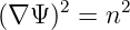
that Ψ satisfies the eiconal equation
and that the surfaces Ψ = constant are wavefronts. We also find that Ψ(P) is double-valued if an
incident and a reflected ray pass through P. These two values of Ψ become equal as P tends
toward the reflecting surface. Thus the reflecting surface is a branch surface of Ψ. If many
rays—incident, reflected, and refracted—pass through P, then Ψ(P) is many-valued, and the
reflecting and refracting surfaces are the branch surfaces on which two or three different branches
are equal.
All the foregoing considerations can also be applied to diffracted rays. We first define the eiconal
Ψ(P) as the optical distance to P from some fixed wavefront measured along any ray, ordinary or
diffracted. We can then show that Ψ still satisfies the eiconal equation. With this new definition
Ψ(P) is even more multiple-valued than before. Not only are the boundaries and discontinuity
surfaces of n(x) branch surfaces of Ψ, but the discontinuity surfaces of derivatives of n(x) are also
branch surfaces. Furthermore the edges and vertices are branch lines and branch points of
Ψ.
In ordinary geometrical optics, in a continuous unbounded medium, it is possible to utilize the
wavefronts and the eiconal equation as a basis for geometrical optics. We prescribe some smooth
surface as an initial wavefront and consider a solution Ψ of the eiconal equation which has the
value zero on the given surface. Because the eiconal equation is quadratic, there are two such
solutions, but they differ from each other only in sign. For either solution we define the surfaces
Ψ = constant as a family of wavefronts and the orthogonal trajectories of these wavefronts
as rays. These rays are exactly the same as the rays given by Fermat’s principle. By
choosing different initial surfaces, we obtain precisely all the rays given by Fermat’s
principle. Thus we see that in this case the wavefront formulation is equivalent to the ray
formulation.
No similar formulation in terms of wavefronts has been given for ordinary geometrical optics in
bounded or discontinuous media. This is undoubtedly due to the occurrence of diffraction in
such media. However, the present theory, which includes diffraction, can presumably be
formulated in terms of wavefronts for any medium. To this end we proceed as above, by
prescribing some smooth surface as an initial wavefront and by considering a solution Ψ of
the eiconal equation which is zero on the given surface. Then we define the surfaces
Ψ = constant to be wavefronts and their orthogonal trajectories to be rays, just as
before.
The only difference is that now we must consider a multiple-valued solution which has as branch
points, lines, and surfaces the vertices, edges, and surfaces determined by the boundaries and by
the refractive index and its derivatives. This solution must be complete, in the sense that it must
branch at every permissible branch point, line, or surface. Unfortunately, the foregoing
requirements do not determine a unique solution Ψ. Other conditions, perhaps at the boundaries or
discontinuity surfaces, must be imposed to obtain uniqueness. Consequently, the equivalence of the
ray and wavefront formulations of our theory is not yet demonstrated, since the wavefront
formulation is not complete.
In two dimensions, an interesting wavefront results from diffraction by an object bounded by a
smooth convex curve. The diffracted wavefronts are the involutes of the curve. In three dimensions,
toroidal wavefronts result from diffraction of a normally incident plane wave by a circular
disk.
6. Imaginary rays
In an unbounded medium in which the refractive index and all its derivatives are continuous, no
diffracted rays occur. This is clear from the above laws governing diffraction. Therefore in such a
medium the theory so far presented coincides with ordinary geometrical optics. However, ordinary
geometrical optics sometimes yields shadows in such media. An example is the region on that side
of a caustic surface through which no rays pass (see Fig. 11). Experimentally some light is
observed in these shadows. Since our theory fails to account for this light, the theory is
incomplete.
To complete the theory, we introduce another new type of ray, which we call an imaginary ray.
Such a ray is a complex-valued solution of the ray equations. Thus, an imaginary ray in a
homogeneous medium is a complex straight line. The definition presupposes that n(x) is analytic
or piecewise analytic. Now we may consider an analytic normal congruence of real rays. By
analytic we mean that the rays of the congruence are analytic functions of two real
parameters. Then complex values of these parameters determine imaginary rays of the same
congruence. Therefore every analytic congruence contains imaginary rays. Some of them will
enter the shadows of the type considered above and thus account for the light observed
there.
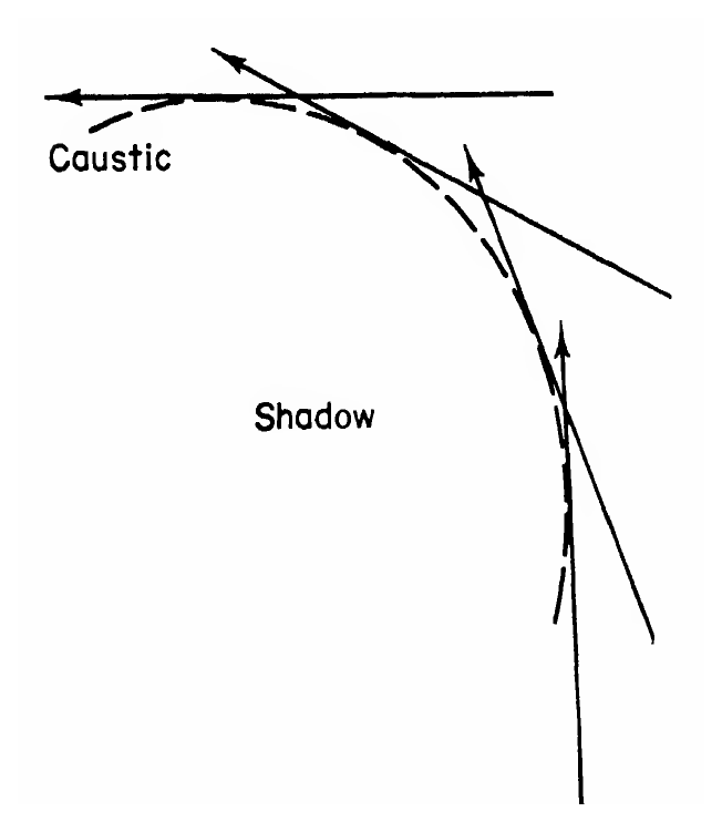
Fig. 11. A set of rays forming a caustic, or envelope. The shadow on one side of the caustic is
devoid of real rays.
To see this, consider a two-dimensional homogeneous medium. Suppose a given curve C is a
caustic, i.e., an envelope of a normal congruence of rays. These rays are then straight lines
tangent to C. Let t denote arc length along C, and let the parametric equations of C be
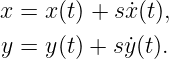
x = x(t), y = y(t). Then the equations of a ray tangent to C at the point [x(t),y(t)]
are
In (1) the parameter s is the signed distance from [x(t),y(t)] on C to (x,y) on the ray.
If the point (x,y) is given, the rays through it are determined by the solutions s,t of (1). Each
solution yields one ray through (x,y). If C is convex, there will generally be two rays through each
point on the convex side of C but no real rays through any point on the concave side. This is
because there are no tangents from such points to C. However, if C is analytic, (1) may have
complex solutions for s and t. Then for each solution s,t the point (x,y) lies on the complex ray
(1) which is tangent to C at the complex point [x(t),y(t)]. The value of s is the complex
distance from (x,y) to the point of tangency, and (x,y) is the only real point on the
ray.
As an example, suppose that C is a circle of radius a. Let the polar coordinates (a,ϕ) denote a
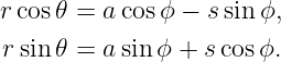
point on C and let (r,𝜃) denote a point off C. Then (1) becomes
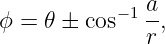
Solving these equations for the point of tangency ϕ and the distance s, we obtain
From (3) we see that, for r ≥ a, there are two real values of ϕ, if cos −1 is restricted to the range 0
to π. There are likewise two real values of t, one corresponding to each value of ϕ. If
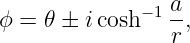
r < a, (3) and (4) do not yield real values of ϕ and s, but they do give the complex
values
Thus two complex straight lines through (r,𝜃) are tangent to the circle r = a at the two points
with ϕ coordinates given by (5). These complex lines are the imaginary rays through (r,𝜃) which
belong to the normal congruence having the circle r = a as caustic.
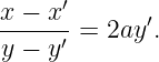
As a second example, consider as caustic the parabola x′ = ay′2. If a line through (x,y) is tangent
to the parabola at (x′,y′), then
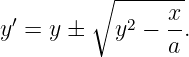
Solving for the point of tangency, we obtain
Equation (8) shows that there are two, one, or no real points of tangency according as (x,y) is
outside, on, or inside the parabola. In the latter case there are two complex points of tangency and
thus two imaginary rays through (x,y). The distance s from (x,y) to the point of tangency is given
in the original paper as
PhysicsLibrary conversion note. Equation (9) above preserves the first factor y2 −x∕2 exactly as printed
in the source. Equations (7)–(8) suggest two typographical anomalies in the printed formula:
the first factor contains x∕2 rather than x∕a, and the last radical term is printed without a
factor of y. Both have been preserved exactly as printed rather than silently altered in this
conversion.
This distance is complex for points inside the parabola.
7. The complex eiconal, or phase, function
An analytic normal congruence of rays may be defined as the set of rays normal to a given analytic
surface S. Such a congruence contains imaginary as well as real rays. By means of the real rays, we
have already defined the real eiconal, or phase, function Ψ(P). This is the optical length to P from
S along a ray of the congruence. Now we may define the complex eiconal Ψ(P) in exactly
the same way by means of the complex rays. It is readily seen that Ψ(P) is complex
and that it satisfies the eiconal equation. Furthermore, it is the analytic continuation
of the real phase function, which is defined only at points P lying on real rays of the
congruence.
In the same way, we can obtain the analytic continuation of the solution of the Cauchy problem for
the eiconal equation. In this problem a surface S, not necessarily a wavefront, is given, and a
function Ψ0 of position on S is also given. We are to find a solution Ψ of the eiconal equation such
that Ψ = Ψ0 on S. This problem is usually solved by means of certain real rays through S. The
analytic continuation can be obtained by applying the same considerations to the imaginary rays
through S.
As an example, let us consider a two-dimensional homogeneous medium with n(x) = 1.
We seek a solution Ψ of the eiconal equation (∇Ψ)2 = 1 having the value Ψ = t on C.
As before, t denotes arc length along C. Since the derivative of Ψ along C is unity,
and since the length of ∇Ψ is unity, we see that ∇Ψ is tangent to C. Therefore the
problem we have posed is a characteristic boundary-value problem, since C is everywhere
characteristic (i.e., tangent to the rays). This problem has two solutions because the eiconal
equation is quadratic. From the eiconal equation the derivative of Ψ along a ray is ±1.
Therefore the solutions are given in terms of the parameters s and t by equations (1)
and
At points (x,y) for which s and t are real, Ψ is also real. However, for points lying on imaginary
rays, both s and t are complex; hence Ψ is complex.
In the case of the circle treated above, s is given by (4) or (6) and t = aϕ, where ϕ is given by (3)
or (5). Then from (10) we have in this case
For the parabola previously considered, if t = 0 at x = y = 0, we find
When this value of t is used in (10), together with s, given by (9), two solutions Ψ result which are
real on and outside the parabola but complex inside it.
Complex solutions of the eiconal equation can also be obtained without making use of imaginary
rays. As an example, consider the above problem for any curve C. Let a(t) be the radius of
curvature of C and ρ be the distance along the normal to C, measured positively toward the
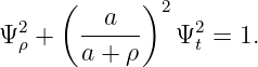
convex side of C. In terms of ρ and t the eiconal equation becomes
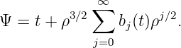
On the basis of the explicit solutions above, we assume that Ψ has the form
Upon inserting (15) into (14) and utilizing the boundary condition on C, we find
The remaining coefficients can be found from a recursion formula which we will omit. The result
(16) shows that Ψ is real for ρ > 0 and complex for ρ < 0, and that the imaginary part of Ψ is
proportional to |ρ|3∕2 for ρ small.
Let us write Ψ = R + iI, where R and I are real. Then the eiconal equation yields
Equation (17) shows that the surfaces R = constant are orthogonal to the surfaces I = constant. In
the next section these surfaces will be shown to be surfaces of constant phase and of constant
amplitude, respectively, for a field associated with Ψ. Thus (17) shows that for this field these
surfaces are mutually orthogonal.
8. Field and amplitude
To make our theory quantitative, we associate a field u(s) with each ray. It is composed of an
amplitude A(s) and a phase Ψ(s) in the form
In (19), k = ω∕c is the propagation constant, determined by the angular frequency ω of the field
and the propagation velocity c in empty space. Equivalently, k = 2π∕λ, where λ is the wavelength
of the field in empty space. Thus our construction applies to a time-harmonic field. The time factor
e−iωt will be omitted. The total field at a point P is the sum of the fields (19) on all rays through
P.
When we deal with light, u is either the electric or the magnetic field and therefore A is a vector.
However, our theory also applies to other types of field (e.g., acoustic pressure). For simplicity we
shall describe it for a scalar u and then indicate the modifications which occur for vector
fields.
We first assume that the phase difference Ψ(P) − Ψ(Q) between two points on a ray is equal to the
optical length L of the ray from Q to P. We also assume that a direction of propagation is
associated with each ray and that Ψ increases in this direction. From these assumptions it follows
that Ψ can be determined at any point P if it is known at some point Q on the same
ray:
We further require that Ψ be constant on some wavefront of a normal congruence of rays. Then Ψ
is just the eiconal, or phase, function previously introduced.
Next we assume that the principle of conservation of energy applies in its optical form. This states
that the energy flux is the same at every cross section of a tube of rays. We assume that the energy
flux per unit area is proportional to nA2. Then the energy principle yields, for a narrow tube of
rays,
Here n and A are evaluated at a point P on a ray in the tube, and dσ is the cross-sectional area of
the tube at P. The quantities n0, A0, and dσ0 are evaluated at some other point Q of the same ray.
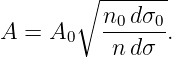
From (21) we obtain
Thus we can compute A at any point P on a ray, provided that we know the amplitude A0 at some
point Q on the same ray. The ratio dσ0∕dσ in (22) is the ratio of the areas of the cross sections at
P and Q. Since these cross sections are portions of wavefronts, this ratio is just the Jacobian of the
mapping from a wavefront at P to that at Q by means of rays. When A is a vector, we
assume that its amplitude satisfies (22). Its direction, if A is an electric or magnetic
field, is obtained from A0 by parallel transport along the ray with respect to the metric
nds.
If ρ1 and ρ2 denote the principal radii of curvature of the wavefront at Q, then, in a homogeneous
medium, the corresponding radii at P are ρ1 + s and ρ2 + s. Here s denotes the distance along the
ray from Q to P. Since the area ratio is inversely proportional to the ratio of Gaussian curvatures,
(22) becomes
From (23) and (20) we see that, in a homogeneous medium,
Here Ψ0 = Ψ(Q).
The field (24) becomes infinite at two, one, or no points on a ray, according as both, one, or neither
of the radii of curvature are finite. These points are on the caustics of the ray congruence. In these
various cases, u decays for large s like s−1, s−1∕2, or s0, that is, as in a spherical, cylindrical, or
plane wave. Later we shall indicate how to modify our theory in order to obtain a finite value for u
on a caustic.
In homogeneous media it is often convenient to measure s from a point Q on the caustic C. To do
this, we first rewrite (23) in the form
The left side of (25) has a limit as Q tends to C, and therefore the right side must also. This is
understandable since A0 becomes infinite and ρ1 becomes zero as Q tends to C. Let us denote this
limit by A′0 = lim Q→CA0ρ11∕2. Then (24) becomes
In a two-dimensional medium, or for cylindrical waves in three dimensions, ρ2 is infinite, and (26)
becomes
In two dimensions, as we have seen, Ψ0 = nt, where t denotes arc length along C. Furthermore,
since A′0 varies from ray to ray, we may designate each ray by its point of tangency t and write
A′0 = A′0(t). Then (27) becomes
If two rays pass through a point P, as is often the case near a caustic, then u(P) is a sum of two
terms of the form (28).
Let us apply (28) to the congruence of rays tangent to a circular caustic of radius a. Making use of
our previous results for s and t, we obtain for r > a,
| u(r,𝜃) = | ![′ − 1
A0[a𝜃-−√-a-cos---(a∕r)]
4 r2 − a2](https://images.physicslibrary.org/cache/objects/1297/make4ht/AGeometricalTheoryOfDiffraction32x.png) eikn[a𝜃−a cos −1(a∕r)+ eikn[a𝜃−a cos −1(a∕r)+ ] ] | |
|
| + ![A ′[a𝜃 + acos−1(a∕r )]
--0---√4-------------
r2 − a2](https://images.physicslibrary.org/cache/objects/1297/make4ht/AGeometricalTheoryOfDiffraction34x.png) eikn[a𝜃+a cos −1(a∕r)− eikn[a𝜃+a cos −1(a∕r)− ]−iπ∕2. ]−iπ∕2. | (29) |
For r < a we also obtain two terms, each corresponding to one of the imaginary rays through the
point (r,𝜃). One of these terms increases with distance from the caustic, whereas the other
decreases. We now assume that the increasing term must be omitted. Then we obtain for
r < a,
For the result (30) we require that A′0(t) be an analytic function of t.
Let us now consider the function v(r,𝜃) defined by
This function is an exact solution of the reduced wave equation in two dimensions if B is a
constant. We now expand it asymptotically for large nka and nkr. This yields exactly (29) for
r > a and (30) for r < a, provided that A′0 is constant and that B = eiπ∕4 A′
0. This
agreement indicates that our construction yields the leading term in the asymptotic expansion with
respect to k, for k large, of the exact solution of the wave equation. We believe that this is always
the case.
A′
0. This
agreement indicates that our construction yields the leading term in the asymptotic expansion with
respect to k, for k large, of the exact solution of the wave equation. We believe that this is always
the case.
So far, we have described how the amplitude varies along a ray. Now we shall explain how the
initial value of the amplitude is to be determined. First, on rays which come from a source—even if
it is at infinity—the amplitude must be prescribed. This prescription characterizes the source.
Second, on a reflected or refracted ray at the point of reflection or refraction, we assume that the
amplitude is proportional to that on the corresponding incident ray at this point. The
proportionality factors are called reflection and transmission coefficients, R and T, respectively. For
vector fields these coefficients are matrices. Third, on a ray diffracted from an edge
or vertex we assume that the field is also proportional to that on the corresponding
incident ray at the point of diffraction. The proportionality factor we call a diffraction
coefficient (or matrix, in the vector case). Additional hypotheses must be made to treat the
fields on diffracted rays which have arcs on boundaries, but we shall not consider them
here.
We assume that the various coefficients just introduced are determined solely by local conditions at
the point of reflection, refraction, or diffraction. Thus, for example, the reflection and transmission
coefficients depend only upon the angle between the incident ray and the surface normal as well as
upon the properties of the media at the point of reflection. Therefore they can be determined from
the solution of a canonical problem, that of reflection and refraction of a plane wave at a plane
interface. The diffraction coefficients can also be obtained from the solutions of appropriate
canonical problems.
The various coefficients depend upon the type of field under consideration. Sound waves will have
different coefficients from water waves, electromagnetic waves, or other waves. Consequently, these
coefficients must be determined separately for different fields. Mathematically, this difference will
be manifested by the differential equations and boundary conditions which occur in the canonical
problems.
Canonical solutions can also be used to modify the results of our theory at and near caustics.
Thus, for example, let us again consider a two-dimensional homogeneous medium in which
a circular caustic occurs. Our results (29) and (30) for the field u become infinite on
the caustic r = a. But the function v in (31), which is asymptotic to u for large k,
remains finite on the caustic. Therefore we can use v instead of u on and near the caustic
in order to obtain a finite value for the field. We can also assume that a finite value
for the field at a point on any caustic can be obtained from the field u off the caustic
by the same correction factor, involving the radius of curvature of the caustic at the
point.
9. Relation to other work
Some types of diffracted rays and diffracted wavefronts have already occurred in the solutions of
particular diffraction problems. Some others have been observed experimentally or have been
introduced to explain particular experimental results. We will now describe some of this previous
work.
First we recall Thomas Young’s proposal that diffraction through an aperture in a screen is an
edge effect. This proposal is in agreement with the present theory, which even makes it precise.
Next we note that Sommerfeld’s solution of Maxwell’s equations for two-dimensional diffraction of
waves by a half plane contains a cylindrical wave emanating from the edge [4]. The cylindrical
wavefronts of this wave are just the diffracted wavefronts, and the normals to these cylinders are
the diffracted rays, of our theory. The solutions of Sommerfeld and Macdonald for two-dimensional
diffraction by wedges also contain cylindrical waves emanating from the edge. Their
solutions for the three-dimensional case contain the cone of diffracted rays from each edge
point.
The bright lines in the shadows of plates, observed by G. G. Becknell and J. Coulson [2, 3] have
already been mentioned and explained in terms of our theory. Later Nijboer observed similar
bright lines in the diffraction patterns of apertures. He introduced diffracted rays emanating
normally from the edge and found that the caustics of these rays were exactly the observed bright
lines.
The present theory predicts the bright spot on the axis of a circular disk, as was noted
above. This result is particularly interesting, because the observation of the bright spot
was a strong argument for the wave theory of light. We now see that this result is also
predicted by a ray theory. Therefore, if this ray theory had been available at the time of the
controversy between ray and wave theory, it might have forestalled the acceptance of the
latter.
The field diffracted through an aperture in a screen can be represented as an integral over the
aperture and screen. Using Kirchhoff’s approximate values for the integrand, A. Rubinowicz [5]
reduced this integral to a line integral along the aperture rim and evaluated it by the method of
stationary phase. The stationary points which he obtained for a given field point P coincide
exactly with the places on the edge at which the diffracted rays through P are produced. N. G. van
Kampen [6] evaluated asymptotically the integrals given by the modified Kirchhoff method.
His result also contains one stationary point corresponding to each edge-diffracted ray
through P, and in addition one stationary point corresponding to each corner of the edge,
accounting for the corner-diffracted rays. R. M. Lewis, B. D. Seckler, and the present author
[7] have obtained similar results from W. Braunbek’s [8] modification of the Kirchhoff
theory.
Surface rays appear in the asymptotic expansion for large ka of the field diffracted by a sphere or
cylinder of radius a. This was originally shown by G. N. Watson and elaborated by B. van der Pol
and H. Bremmer [9], B. Friedman [10], I. Imai [11], W. Franz [12], and others. The tangent rays
shed by these surface rays are exhibited in the exact solution of W. Franz [12] and the
approximate solution of W. Franz and K. Depperman [13]. The latter authors showed that
calculations of radar reflection from cylinders, based on the idea of surface rays, agreed
excellently with the measurements of Limbach. F. G. Friedlander [14] introduced surface
rays and the associated wavefronts in studying diffraction by cylinders of convex cross
section.
Surface rays produced by refraction at the critical angle occur in the work of E. Gerjuoy [15] and of
L. Brekovskih [16]. These authors examined the field produced by a point source near a plane
interface between two media, in the high-frequency limit. They found that each critically refracted
ray gave rise to the appropriate diffracted rays. Such rays have been observed experimentally in
acoustics.
Spherical waves emanating from the tip occur in the solution for the field diffracted by a
circular or elliptic cone. The wavefronts and rays of these waves are just the diffracted
wavefronts and rays predicted by the theory in this case. The rays leave the vertex in all
directions.
Rays reflected from surfaces of discontinuity of derivatives of the index of refraction do
not seem to have been considered before. However, the fact that such discontinuities
do reflect at normal incidence was noticed by J. Feinstein [17] and S. A. Schelkunoff
[18].
The possibility of using rays in a systematic way for the calculation of fields was investigated by R.
K. Luneberg [19]. He suggested that the ray construction would yield the leading term in the
asymptotic expansion of the field for large k. The procedure for obtaining further terms in this
asymptotic expansion was given by M. Kline [20], both for Maxwell’s equations and for more
general equations. Other authors have considered the same type of expansion for various
equations. Thus F. G. Friedlander [21], H. Bremmer [22], and E. T. Copson [23] also
considered Maxwell’s equations; S. C. Lowell [24] considered waves in shallow water; J.
B. Keller [25] considered weak shock waves; G. D. Birkhoff [26], L. Brillouin [27], G.
Wentzel [28], P. A. M. Dirac [29], and J. B. Keller [30] considered the Schroedinger
equation of quantum mechanics; F. G. Friedlander and J. B. Keller [31] considered
the reduced wave equation; and W. J. Trjitzinsky [32] considered a very general linear
equation. All of these authors restricted their attention to the rays of ordinary geometrical
optics.
Many diffraction problems have been solved with the ray method by C. Schensted [33], J. B.
Keller, R. M. Lewis, and B. D. Seckler [34], J. B. Keller [25, 30, 35, 36], K. O. Friedrichs and J.
B. Keller [37], B. R. Levy and J. B. Keller [38], S. N. Karp and J. B. Keller [39], B. D.
Seckler and J. B. Keller [41], etc. Whenever possible, the fields constructed by the ray
method were compared with asymptotic expansions (for large k) of exact solutions. In
all such cases perfect agreement was obtained. In other cases numerical results were
compared, and good agreement was obtained for ka ≥ 2, where a is a typical length in the
problem.
All of these results suggest that the ray method does yield the leading terms in the
asymptotic expansions of solutions of diffraction problems. However, a general proof of this
statement has not yet been obtained. Partial results of this kind are given by R. K.
Luneberg [19], M. Kline [20], W. J. Trjitzinsky [32], W. L. Miranker [40], and R. M. Lewis
[42].
PhysicsLibrary source note. This PhysicsLibrary entry is a conversion of the public-domain
material in Reference [1].
References
References
[1] J. B. Keller, “A Geometrical Theory of Diffraction,” in L. M. Graves (ed.), Calculus
of Variations and Its Applications, Proceedings of Symposia in Applied Mathematics,
Vol. VIII, McGraw-Hill Book Company, Inc., for the American Mathematical Society,
1958, pp. 27–52.
[2] J. Coulson and G. G. Becknell, “Reciprocal diffraction relations between circular
and elliptical plates,” Phys. Rev., vol. 20 (1922), p. 594.
[3] J. Coulson and G. G. Becknell, “An extension of the principle of the diffraction
evolute and some of its structural detail,” Phys. Rev., vol. 20 (1922), p. 607.
[4] A. J. W. Sommerfeld, Optics, Academic Press, Inc., New York, 1954.
[5] A. Rubinowicz, “The diffraction waves in Kirchhoff’s theory of diffraction
phenomena,” Ann. Phys., vol. 53 (1917), p. 257.
[6] N. G. van Kampen, “An asymptotic treatment of diffraction problems,” Physica,
vol. 14 (1949), p. 575.
[7] J. B. Keller, R. M. Lewis, and B. D. Seckler, “Diffraction by an aperture, II,” New
York Univ. Inst. Math. Sci. Research Rep. EM-96 (1956); J. Appl. Phys., vol. 28, no. 5
(May 1957), pp. 570–579.
[8] W. Braunbek, “Neue Näherungsmethode für die Beugung am ebenen Schirm,”
Zeit. Physik, vol. 127 (1950), p. 381; “Zur Beugung an der Kreisscheibe,” Zeit. Physik,
vol. 127 (1950), p. 405.
[9] H. Bremmer, Terrestrial Radio Waves, Elsevier Press, Inc., Houston, 1949.
[10] B. Friedman, Comm. Pure Appl. Math., vol. 4 (1951), p. 317.
[11] I. Imai, “Die Beugung electromagnetischer Wellen an einem Kreiszylinder,” Zeit.
Physik, vol. 137 (1954), pp. 31–48.
[12] W. Franz, Zeit. Natur., vol. 9a (1954), pp. 705–716.
[13] K. Depperman and W. Franz, “Theorie der Beugung an der Kugel unter
Berücksichtigung der Kriechwelle,” Ann. Phys., Ser. 6, vol. 14 (1954), pp. 253–264.
[14] F. G. Friedlander, Proc. Cambridge Philos. Soc., vol. 38 (1942), p. 383.
[15] E. Gerjuoy, Comm. Pure Appl. Math., vol. 6 (1953), p. 73.
[16] L. Brekovskih, Tech. Phys. USSR, vol. 18 (1948), p. 455.
[17] J. Feinstein, Trans. IRE, PGAP, AP-2 (1954), p. 23.
[18] S. A. Schelkunoff, Comm. Pure Appl. Math., vol. 4 (1951), p. 181.
[19] R. K. Luneberg, The Mathematical Theory of Optics, Brown University, 1944;
Propagation of Electromagnetic Waves, New York University, 1948.
[20] M. Kline, “An asymptotic solution of Maxwell’s equations,” Comm. Pure Appl.
Math., vol. IV, no. 2–3 (August 1951), pp. 225–263; “Asymptotic solution of linear
hyperbolic partial differential equations,” J. Rational Mech. Anal., vol. 3, no. 3 (May
1954).
[21] F. G. Friedlander, “Geometrical optics and Maxwell’s equations,” Proc. Cambridge
Philos. Soc., vol. 43, part 2 (1946), pp. 284–286.
[22] H. Bremmer, “The jumps of discontinuous solutions of the wave equation,” Comm.
Pure Appl. Math., vol. IV, no. 4 (November 1951), pp. 419–427.
[23] E. T. Copson, “The transport of discontinuities in an electromagnetic field,” Comm.
Pure Appl. Math., vol. IV, no. 4 (November 1951), pp. 427–435.
[24] S. C. Lowell, “The propagation of waves in shallow water,” Comm. Pure Appl. Math.,
vol. 2, no. 2–3 (1949), pp. 275–291.
[25] J. B. Keller, “Geometrical acoustics, I, The theory of weak shocks,” J. Appl. Phys.,
vol. 25, no. 8 (August 1954), pp. 938–947.
[26] G. D. Birkhoff, “Some remarks concerning Schroedinger’s wave equation,” Proc. Nat.
Acad. Sci. U.S.A., vol. 19 (1933), pp. 339–344; and in Collected Mathematical Papers,
Vol. II, American Mathematical Society, 1950, pp. 813–818; “Quantum mechanics and
asymptotic series,” Amer. Math. Soc. Bull., vol. 39 (1933), pp. 681–700; and in Collected
Mathematical Papers, Vol. II, American Mathematical Society, 1950, pp. 837–856.
[27] L. Brillouin, “Remarques sur la mécanique ondulatoire,” J. Phys. Radium, vol.
7 (1936), pp. 353–368; “La mécanique ondulatoire; une méthode générale de
résolution par approximations successives,” C. R. Acad. Sci. Paris, vol. 183 (1926), p.
24.
[28] G. Wentzel, “Eine Verallgemeinerung der Quantenbedingungen für die Zwecke der
Wellenmechanik,” Zeits. Physik, vol. 38 (1926), p. 518.
[29] P. A. M. Dirac, The Principles of Quantum Mechanics, Oxford University Press,
London, 3rd ed., 1947, pp. 121–123.
[30] J. B. Keller, “Derivation of the Bohr-Sommerfeld quantum conditions from an
asymptotic solution of the Schroedinger equation,” New York Univ. Inst. Math. Sci.
Research Rept. CX-10 (July 1953).
[31] F. G. Friedlander and J. B. Keller, “Asymptotic expansions of solutions of (∇2 +
k2)u = 0,” New York Univ. Inst. Math. Sci. Research Rep. EM-67 (September 1954);
Comm. Pure Appl. Math., vol. 8, no. 3 (August 1955), pp. 387–394.
[32] W. J. Trjitzinsky, “Analytic theory of parametric linear partial differential
equations,” Rec. Math., vol. 15 (1944), p. 179.
[33] C. Schensted, “The electromagnetic transport equation and the Luneberg-Kline
method of solution,” Univ. of Michigan, Eng. Research Inst. Rep. 15-25-(504)-3.
[34] J. B. Keller, R. M. Lewis, and B. D. Seckler, “Asymptotic solution of some diffraction
problems,” New York Univ. Inst. Math. Sci. Research Rep. EM-81 (1955); Comm. Pure
Appl. Math., vol. 9 (1956), p. 207.
[35] J. B. Keller, “Diffraction by an aperture, I,” New York Univ. Inst. Math. Sci.
Research Rept. EM-92 (1956); J. Appl. Phys., vol. 28, no. 4 (April 1957), pp. 426–444.
[36] J. B. Keller, Trans. IRE, PGAP, AP-4 (1956), pp. 312–321.
[37] K. O. Friedrichs and J. B. Keller, “Geometrical acoustics, II; Diffraction, reflection
and refraction of a weak spherical or cylindrical shock at a plane interface,” J. Appl.
Phys., vol. 26 (1955), pp. 961–966.
[38] J. B. Keller and B. Levy, “Diffraction by a smooth object,” to be published, New
York Univ. Inst. Math. Sci. EM Series; B. R. Levy and J. B. Keller, “Diffraction by
a smooth object,” New York Univ. Inst. Math. Sci. Research Rep. EM-109 (December
1957).
[39] S. N. Karp and J. B. Keller, “Diffraction by an aperture, III,” to be published, New
York Univ. Inst. Math. Sci. EM Series.
[40] W. L. Miranker, “The asymptotic theory of solutions of Δu + k2u = 0,” New York
Univ. Inst. Math. Sci. BR-21 (1956).
[41] B. D. Seckler and J. B. Keller, “Diffraction in inhomogeneous media,” New York
Univ. Inst. Math. Sci. Research Rep. MME-7 (December 1957).
[42] R. M. Lewis, “Discontinuous initial value problems and asymptotic expansion
of steady-state solution,” New York Univ. Inst. Math. Sci. Research Rep. MME-8
(December 1957).
Institute of Mathematical Sciences, New York University, New York, N.Y.

![∫
Q
L = n[x(s)]ds.
P](https://images.physicslibrary.org/cache/objects/1297/make4ht/AGeometricalTheoryOfDiffraction2x.png)





![[ ( ) √-------]
Ψ = a𝜃 ∓ i a cosh−1 a- − a2 − r2 , r ≤ a.
r](https://images.physicslibrary.org/cache/objects/1297/make4ht/AGeometricalTheoryOfDiffraction15x.png)

![[ ∘ -- ]
3∕2 2- 2- ˙a--1∕2 ˙a2 −-3a¨a-−-27-
Ψ = t + ρ 3 a + 6aρ + √ -- 3∕2 ρ + ⋅⋅⋅ .
45 2 a](https://images.physicslibrary.org/cache/objects/1297/make4ht/AGeometricalTheoryOfDiffraction19x.png)





![[ ]
ρ1ρ2 1∕2
A = A0 ---------------- .
(ρ1 + s)(ρ2 + s)](https://images.physicslibrary.org/cache/objects/1297/make4ht/AGeometricalTheoryOfDiffraction26x.png)
![[ ]1∕2
------ρ1ρ2------ ik(Ψ0+ns)
u(s) = (ρ1 + s)(ρ2 + s) A0e .](https://images.physicslibrary.org/cache/objects/1297/make4ht/AGeometricalTheoryOfDiffraction27x.png)
![[ −1]1∕2 1∕2
A (ρ1 + s)(ρ2 + s )ρ 2 = A0 ρ1 .](https://images.physicslibrary.org/cache/objects/1297/make4ht/AGeometricalTheoryOfDiffraction28x.png)
![[ ]1∕2
u(s) = ----ρ2--- A ′eik(Ψ0+ns).
s(ρ2 + s) 0](https://images.physicslibrary.org/cache/objects/1297/make4ht/AGeometricalTheoryOfDiffraction29x.png)


![A-′0[a-𝜃 +-ai-cosh−1(a∕r)] kn[ia𝜃+acosh−1(a∕r)−√a2−r2]−iπ∕4
u(r,𝜃) = √4a2--−-r2 e .](https://images.physicslibrary.org/cache/objects/1297/make4ht/AGeometricalTheoryOfDiffraction36x.png)
![[ (1) (2) ] inka𝜃
v (r,𝜃) = B Hnka(nkr ) − H nka(nkr ) e .](https://images.physicslibrary.org/cache/objects/1297/make4ht/AGeometricalTheoryOfDiffraction37x.png)