Wave Mechanics: Power Carried by a 1D Wave
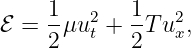
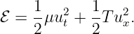
WM18 developed the mechanical energy density of an ideal stretched string,
Energy density answers the question, “How much mechanical energy is stored near this position?”
The next question is different:
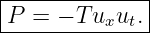
That rate of energy transfer is the wave power. With positive power defined as energy flow toward
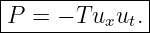
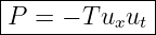
increasing x, the ideal-string result is
The sign matters. A positive value means net mechanical energy crosses the chosen position toward
+x; a negative value means the net flow is toward −x. This local expression is the one-dimensional
energy-flux law associated with the string wave equation and is consistent with standard
wave-energy treatments [1, 2, 3, 4].
WM19 derives the result mechanically and from local energy conservation, applies it to arbitrary
traveling profiles and sinusoidal waves, derives the time-averaged sinusoidal power, and explains
what happens when right- and left-moving waves are both present.
1 Power is energy crossing a position per unit time
Choose a fixed position x. During a short time interval dt, mechanical energy can cross that
position even though the material of the string merely oscillates transversely.
We define P(x,t) so that
means energy transport toward increasing x, and
means energy transport toward decreasing x.
The SI unit of power is
This is not yet intensity. Intensity is power per unit area and will be introduced later when waves
spread through higher-dimensional space [3].
2 Mechanical derivation at a cut in the string
Imagine cutting the mathematical description of the string at one fixed position. The material just
to the left exerts a Tension force on the material just to the right.
For a small-slope string, the transverse component of the force exerted by the left side on the right
side is approximately
The transverse velocity of the material at the cut is
Mechanical power delivered from the left portion into the right portion is force times
velocity:
| P | = Fuvu | (8)
|
| = (−Tux)ut. | (9) |
Therefore
The geometry and sign convention are summarized below.

Figure. At a fixed cut, the local slope determines the transverse component of tension and
ut gives the local material velocity. Their product determines the mechanical work rate
across the cut. Positive P is defined as energy transport toward +x.
3 Dimensional check
The tension has units of newtons,
while ux is dimensionless and
Hence
| [Tuxut] | = N | (13)
|
| =  | (14)
|
| = W. | (15) |
So the expression has the correct dimensions for power.
4 The same result from local energy conservation
The energy-density formula from WM18 is
Differentiate with respect to time:
For the ideal string,
Substitute this into the first term:
| ℰt | = Tutuxx + Tuxuxt | (19)
|
| = T (utux). (utux). | (20) |
Therefore
Identifying
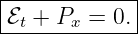
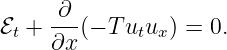
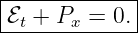
gives the local conservation law
This compact equation says that a local change in stored energy is caused by an imbalance of
power flow into and out of the region.
5 Energy balance on a finite interval
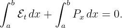
Integrate the local conservation law from x = a to x = b:
Thus
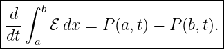
Equivalently,
Power entering at the left boundary increases the energy stored in the interval; power leaving at
the right boundary decreases it.
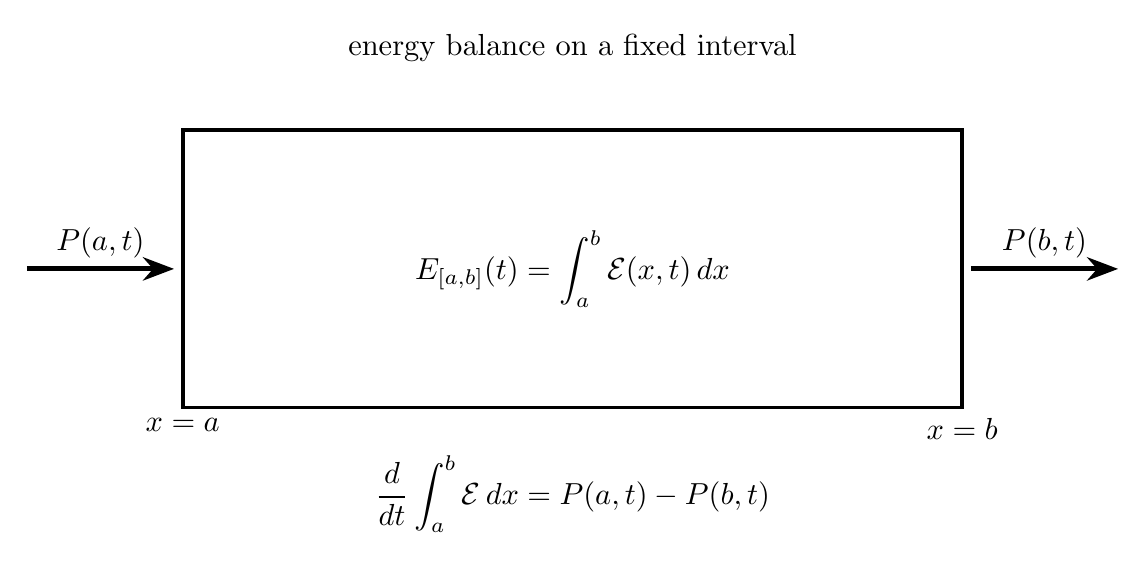
Figure. Energy conservation on a fixed interval: rate of change of stored energy equals
incoming power minus outgoing power.
6 Power in a pure right-moving wave
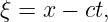
Consider
With
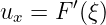
we have
and
Therefore
| P | = −Tuxut | (31)
|
| = −TF′(ξ)[−cF′(ξ)] | (32)
|
| = Tc[F′(ξ)]2. | (33) |
Hence
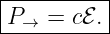
The power is nonnegative because this wave carries energy toward +x.
WM18 showed that the energy density of the same wave is
Therefore
This is physically intuitive: a packet of energy density ℰ translating at speed c carries energy past
a fixed point at rate cℰ.
7 Power in a pure left-moving wave
For
we have
and
Thus
Since
we can write
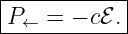
The sign is a direction marker: the energy moves toward decreasing x.
8 Sinusoidal traveling wave
Consider the right-moving sinusoidal wave
Define
Then
and
The instantaneous power is therefore
| P | = −T(−Ak sin 𝜃)(Aω sin 𝜃) | (47)
|
| = TA2kω sin 2𝜃. | (48) |
Hence
It is always nonnegative for this right-moving wave.
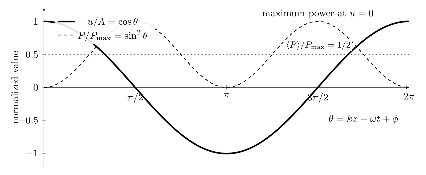
Figure. For a right-moving sinusoidal wave, normalized instantaneous power varies as
sin 2𝜃. Power is largest where the displacement passes through zero and vanishes at
displacement extrema.
9 Average power of a sinusoidal wave
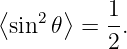
Over one phase cycle,
Therefore
Use
and
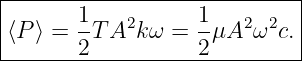
Then
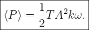
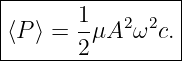
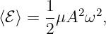
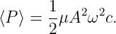
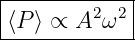
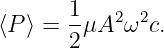
This is the standard time-averaged power of a sinusoidal transverse wave on an ideal string
[3, 1].
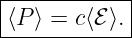
Because WM18 found
we again have
10 Square-law scaling
For a fixed string and a sinusoidal traveling wave,
Thus
when the string properties are fixed.
Consequently:
- doubling A multiplies average power by 4;
- doubling f or ω multiplies average power by 4;
- doubling both amplitude and frequency multiplies average power by 16.
OpenStax emphasizes this same amplitude-squared and frequency-squared scaling for sinusoidal
mechanical waves [3].
11 Both propagation directions at once
For the general two-direction solution
let
Then
and
Substitute into the power law:
| P | = −T[F′ + G′][−cF′ + cG′] | (63)
|
| = Tc![( )
[F ′]2 − [G ′]2](https://images.physicslibrary.org/cache/objects/1185/make4ht/WaveMechanicsPowerCarriedByA1DWave53x.png) . . | (64) |
Thus
The net power is the right-moving contribution minus the left-moving contribution.

Figure. Directional power adds with a sign. Right-moving energy contributes positive
power and left-moving energy contributes negative power under the chosen convention.
12 Standing waves and zero average transport
A Standing Wave can be written
Then
and
Therefore
| P | = −Tuxut | (69)
|
| = TB2kω cos(kx) sin(kx) cos(ωt) sin(ωt). | (70) |
Using double-angle identities,
The instantaneous local power is generally not zero. Its sign reverses as energy moves back and
forth within the standing-wave pattern.
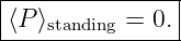
However, over a complete time cycle,
so
A perfect standing wave therefore has no net time-averaged transport through a fixed position,
even though energy can flow locally and instantaneously.
13 Worked Example 1: Power from local slope and velocity
A string has tension
At one event,
Find the instantaneous power and interpret its sign.
Solution
Use
Then
| P | = −(100)(0.020)(−0.30) | (77)
|
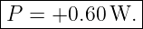
| = 0.60 W. | (78) |
Thus
The positive sign means net energy is crossing the selected position toward increasing x at that
instant.
14 Worked Example 2: Average power of a sinusoidal wave
A right-moving sinusoidal wave has
on a string with
Find c, ω, k, and the time-averaged power.
Solution
The wave speed is
| c | =  | (82)
|
| =  | (83)
|
| ≃ 63.25 m/s. | (84) |
The angular frequency is
Then
| k | =  | (86)
|
| ≃ 0.993 rad/m. | (87) |
Convert the amplitude:
Now use
Thus
| ⟨P⟩ | =  (0.020)(0.0050)2(62.83)2(63.25) (0.020)(0.0050)2(62.83)2(63.25) | (90)
|
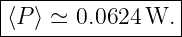
| ≃ 6.24 × 10⁻² W. | (91) |
Therefore
15 Worked Example 3: Required amplitude for a desired average power
A sinusoidal traveling wave moves on a string with
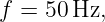
At frequency
what amplitude is required to carry an average power of
Solution
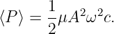
Start with
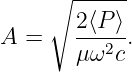
Solve for A:
The angular frequency is
Therefore
| A | = 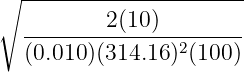 | (99)
|
| ≃ 1.42 × 10⁻² m. | (100) |
Thus
16 Worked Example 4: Power carried by a translating pulse from its energy density
At one location in a pure right-moving pulse, the instantaneous energy density is
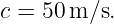
The pulse speed is
Find the instantaneous power at that event.
Solution
For a pure right-moving wave,
Therefore
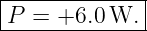
| P | = (50)(0.12) | (105)
|
| = 6.0 W. | (106) |
Hence
If the same energy-density profile were traveling toward −x, the power would instead be
−6.0 W.
17 Worked Example 5: Net power with two propagation directions
At one event in a two-direction wave field, suppose
and the directional profile derivatives have values
Find the net power.
Solution
Use
Then
| P | = (50)(40)![[(0.060)2 − (0.040)2]](https://images.physicslibrary.org/cache/objects/1185/make4ht/WaveMechanicsPowerCarriedByA1DWave90x.png) | (111)
|
| = 2000(0.0036 − 0.0016) | (112)
|
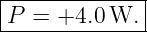
| = 4.0 W. | (113) |
Thus
The right-moving contribution is larger than the left-moving contribution, so the net energy
transport is toward +x.
18 Worked Example 6: Instantaneous power in a standing wave
Consider
with
Find the power at
when
Also state the time-averaged power at that position.
Solution
Because
we have
The standing-wave power is
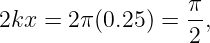
At x = 0.25 m,
so
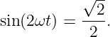
Also
so
Therefore
| P | =  (60)(0.010)2(π)(30π) (60)(0.010)2(π)(30π) | (126)
|
| ≃ 0.314 W. | (127) |
Thus
at this instant.
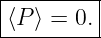
Over a complete oscillation cycle,
The local energy flow reverses later in the cycle, so there is no net time-averaged transport through
the point.
19 Common mistakes
- Mistake: dropping the minus sign in P = −Tuxut. The sign carries
propagation-direction information.
- Mistake: assuming positive displacement means positive power. Power depends on
slope and velocity, not displacement alone.
- Mistake: treating a standing wave as having zero instantaneous power everywhere.
Its time-averaged net transport is zero, but instantaneous local power can be nonzero.
- Mistake: confusing power with energy density. Their units differ: watts versus joules
per meter.
- Mistake: confusing one-dimensional power with intensity. Intensity requires division
by an area.
- Mistake: applying P = cℰ to an arbitrary superposition. That relation holds directly
for a single pure right-moving wave; a left-moving wave gives P = −cℰ, and a
two-direction field requires the signed difference of the directional contributions.
20 Summary
For an ideal stretched string, the instantaneous mechanical power crossing a fixed position
is
Together with
it satisfies the local conservation law
For pure traveling waves,
For a right-moving sinusoidal wave,
and
The next step is to turn these results into a systematic treatment of average power, intensity, and
wave impedance.
References
References
[1] A. P. French, Vibrations and Waves, M.I.T. Introductory Physics Series, W. W.
Norton & Company, 1971.
[2] Frank S. Crawford, Jr., Waves, Berkeley Physics Course, Volume 3, McGraw-Hill,
1968.
[3] William Moebs, Samuel J. Ling, and Jeff Sanny, University Physics, Volume 1,
OpenStax, 2016, Section 16.4, “Energy and Power of a Wave.”
[4] Howard Georgi, The Physics of Waves, Benjamin/Cummings, 1992, continuum and
traveling-wave chapters; also distributed through MIT OpenCourseWare 8.03SC.
[5] Massachusetts Institute of Technology, 8.03SC Physics III: Vibrations and Waves,
Fall 2016, mechanical-wave lectures, notes, and Problem Set 5, MIT OpenCourseWare.
[6] Richard P. Feynman, Robert B. Leighton, and Matthew Sands, The Feynman Lectures
on Physics, Volume I, Chapter 47, “Sound. The wave equation.”







![[T ] = N,](https://images.physicslibrary.org/cache/objects/1185/make4ht/WaveMechanicsPowerCarriedByA1DWave8x.png)
![[ut] = m/s.](https://images.physicslibrary.org/cache/objects/1185/make4ht/WaveMechanicsPowerCarriedByA1DWave9x.png)





![|-----------′--------2-----|
-P→--=-T-c[F-(x-−-ct)]-≥--0.|](https://images.physicslibrary.org/cache/objects/1185/make4ht/WaveMechanicsPowerCarriedByA1DWave26x.png)
![′ 2
ℰ = T[F (x − ct)].](https://images.physicslibrary.org/cache/objects/1185/make4ht/WaveMechanicsPowerCarriedByA1DWave27x.png)



![|----------------------------|
| ′ 2 |
-P←--=-−-T-c[G-(x-+-ct)]-≤--0.](https://images.physicslibrary.org/cache/objects/1185/make4ht/WaveMechanicsPowerCarriedByA1DWave32x.png)
![′ 2
ℰ = T[G (x + ct)],](https://images.physicslibrary.org/cache/objects/1185/make4ht/WaveMechanicsPowerCarriedByA1DWave33x.png)











![|--------------------------------------|
|P = Tc ([F ′(x − ct)]2 − [G ′(x + ct)]2) .|
---------------------------------------](https://images.physicslibrary.org/cache/objects/1185/make4ht/WaveMechanicsPowerCarriedByA1DWave54x.png)




















![( ′2 ′2)
P = T c [F ] − [G ] .](https://images.physicslibrary.org/cache/objects/1185/make4ht/WaveMechanicsPowerCarriedByA1DWave89x.png)