Strapdown Inertial Navigation Examples: Earth Rotation and Navigation Frames
This companion to INS06 turns the frame geometry into calculations that can be checked
by hand and then reused as software unit tests. The emphasis is on transformations
among ECI, ECEF, and local NED coordinates, Earth rate, transport rate, geodetic
position kinematics, and the frame-rate subtraction required by strapdown attitude
propagation.
The notation follows the main INS series. A passive direction cosine matrix Cab transforms
components from frame a into frame b,
and ωabc denotes the angular velocity of frame b relative to frame a, resolved in frame
c.
The WGS-84 constants used throughout are
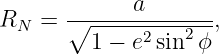
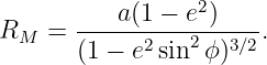
The ellipsoidal radii of curvature are
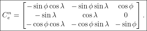
For the local NED frame,
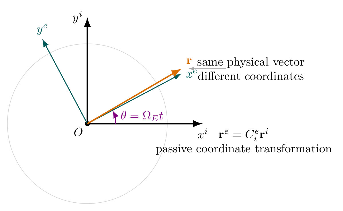
Figure. ECI and ECEF share the same origin but not the same orientation. A passive
coordinate transformation changes the components used to describe a physical vector while
leaving the physical vector unchanged.
1 Exercises
Exercise 1: An inertially fixed position observed in ECEF
At t = 0, let ECI and ECEF axes coincide. An inertially fixed point has
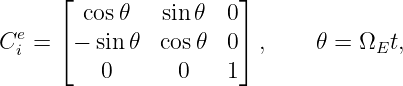
After t = 1800 s, use
to:
- compute the Earth rotation angle 𝜃;
- compute re = C
ieri;
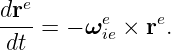
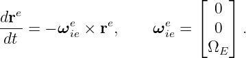
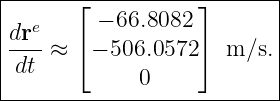
- show that an inertially fixed vector has the ECEF coordinate derivative
Exercise 2: Transforming an ECEF velocity into NED
At
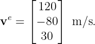
a velocity is represented in ECEF coordinates as
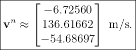
- Construct Cen.
- Compute vn = C
enve.
- Verify that the transformation preserves vector magnitude.
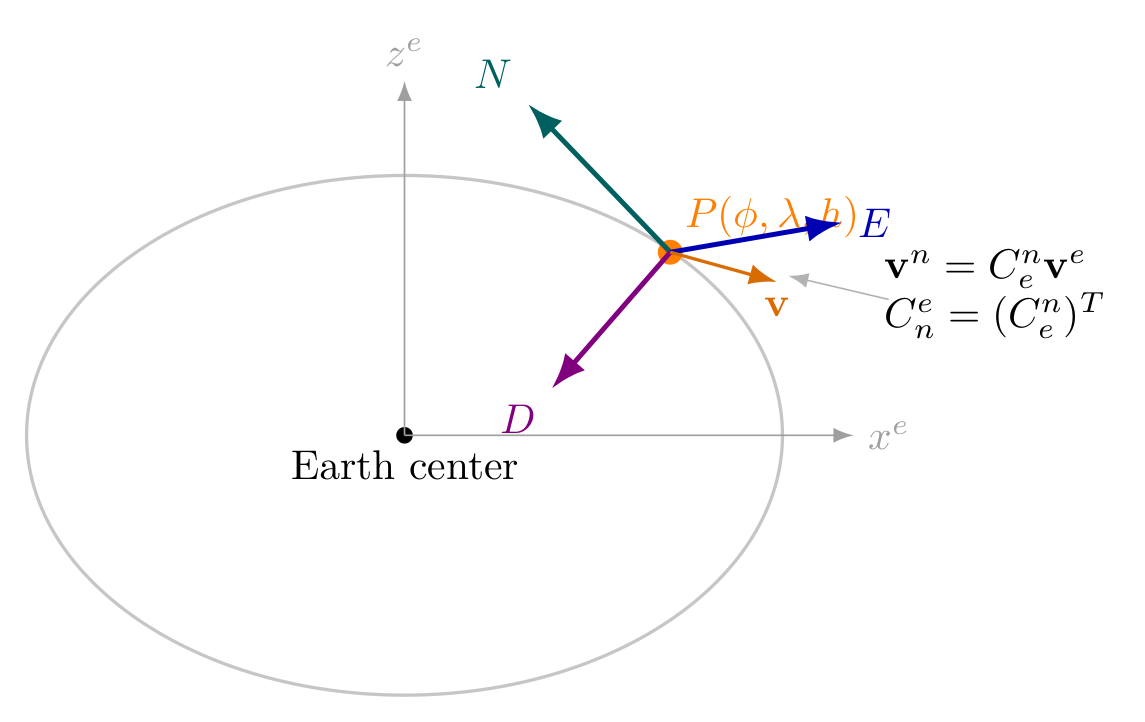
Figure. The local NED axes are a basis attached to the geodetic position. ECEF and NED
coordinates describe the same physical vector using different basis vectors.
Exercise 3: Earth rate in NED and in a yawed body frame
A level vehicle is stationary at geodetic latitude
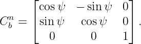
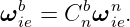
Its heading is ψ = 60∘, measured clockwise from North. For a level vehicle use
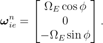
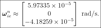
- Compute ωien.
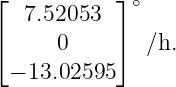
- Express the components in degrees per hour.
- Compute the same Earth-rate vector in body coordinates,
- Explain why the physical rate has not changed even though all three components
changed.
Exercise 4: Transport rate for a moving vehicle
At
a vehicle has
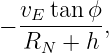
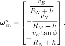
Compute RM, RN, and
Express the result in both rad/s and degrees per hour, and compare its magnitude with the Earth
rotation rate.
Exercise 5: Geodetic position rates
Continue Exercise 4 and let
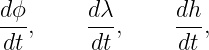
Compute
and express latitude and longitude rates in degrees per hour.
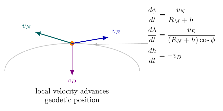
Figure. North, east, and down velocity components drive latitude, longitude, and height
rates through the local ellipsoid geometry.
Exercise 6: From inertial gyro rate to body rate relative to NED
Continue Exercises 4 and 5. The vehicle remains level with heading
Its body executes an additional yaw rotation relative to NED of
about body down. Assume no roll or pitch rate relative to NED.
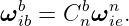
- Compute
- Transform the reference-frame rate into body coordinates.
- Construct the ideal gyro measurement ωibb.
- Recover ωnbb using the strapdown reference-rate subtraction.
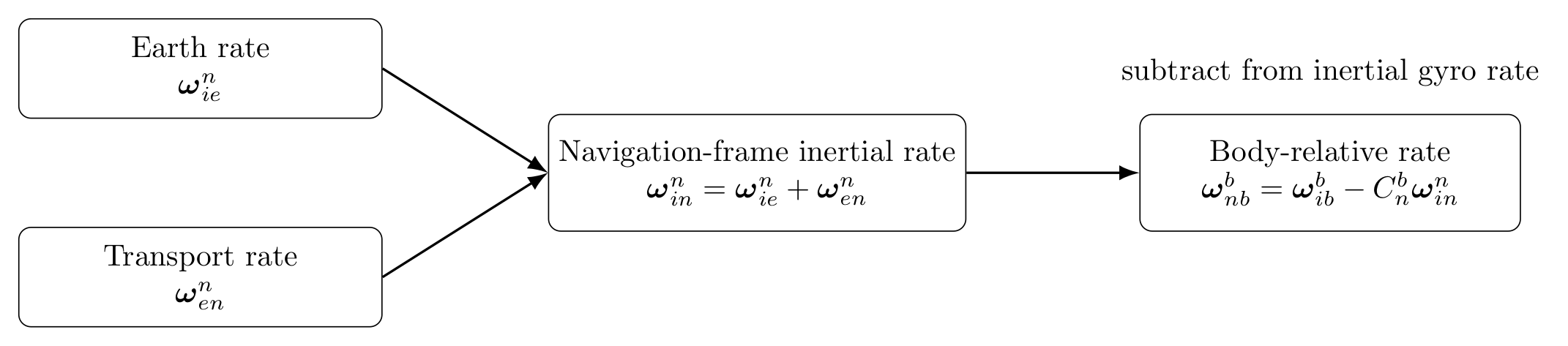
Figure. Earth rate and transport rate combine to form the inertial angular rate of the
navigation frame. That reference rate must be transformed to body axes before it is
subtracted from the inertial gyro measurement.
Exercise 7: DCM chain and round-trip consistency
At
a level vehicle has heading ψ = 45∘.
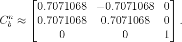
- Construct Cen and C
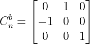
bn.
- Form
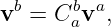
- Transform the body-frame forward velocity
into ECEF.
- Transform the ECEF result back to NED and verify that it matches the direct body-to-NED
transformation.
- Check det Cbe and (C
be)T C
be.
Exercise 8: Derivative consistency between ECEF and NED
At
use
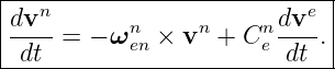
The derivative relation is
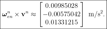
- Compute ωenn × vn.
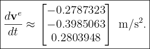
- Solve for dve∕dt.
- Substitute the result back into the NED derivative equation and verify the original
dvn∕dt.
- Explain why simply applying Cen to dve∕dt would be incorrect.
Exercise 9: Stationary Earth-fixed attitude consistency
A level vehicle is fixed to Earth at
with heading ψ = 90∘. Since the vehicle is stationary relative to ECEF,
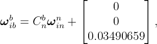
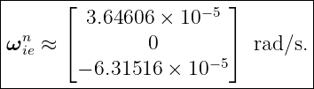
- Compute ωien.
- Compute the ideal gyro measurement
- Show that
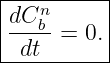
- Verify that the two terms in
are equal, giving dCbn∕dt = 0.
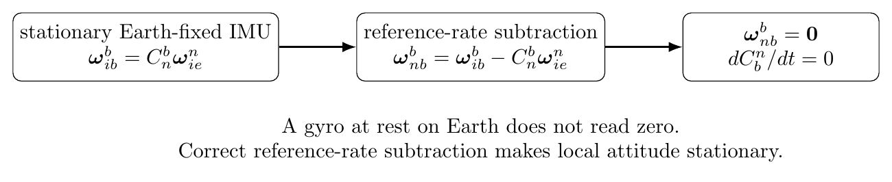
Figure. A stationary Earth-fixed gyro measures Earth rotation. Correct subtraction of the
navigation-frame inertial rate produces zero body rate relative to local NED and therefore
constant local attitude.
Exercise 10: Why local NED becomes ill-conditioned near the poles
At
a vehicle travels due east at
- Compute RN.
- Compute dλ∕dt and express it in degrees per hour.
- Compute ωenn.
- Identify the component that becomes large as ϕ → 90∘.
- Explain why this is a coordinate-frame problem rather than a physical singularity in
the vehicle motion.
2 Worked solutions
Solution 1: An inertially fixed position observed in ECEF
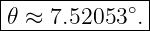
The Earth rotation angle after 1800 s is
Therefore
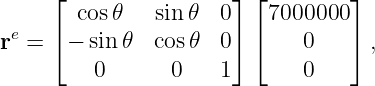
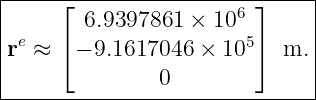
The ECEF components are
so
The point is fixed in ECI, but ECEF rotates underneath it. Hence its ECEF coordinate derivative
is
The cross product gives
This result is a useful reminder that a coordinate derivative can be nonzero even when the physical
vector is fixed in inertial space.
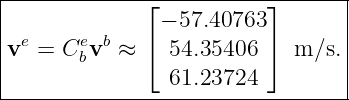
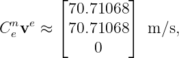
Solution 2: Transforming an ECEF velocity into NED
For ϕ = 40∘ and λ = −105∘,
Then
which gives
The negative down component means the velocity has an upward component of about 54.7
m/s.
Because Cen is orthogonal,
Numerically,
This is one of the simplest and most useful DCM implementation checks.
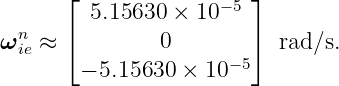
Solution 3: Earth rate in NED and in a yawed body frame
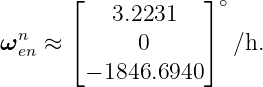
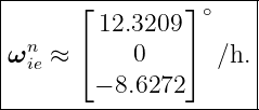
Earth rate in NED is
At 35∘,
In degrees per hour,
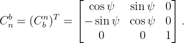
For ψ = 60∘,
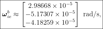
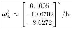
Thus
or
The physical angular-velocity vector has not changed. Only its coordinate components changed
because the basis changed from NED to body axes.
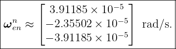
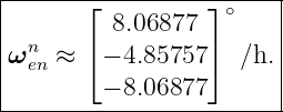
Solution 4: Transport rate for a moving vehicle
At 45∘ latitude,
Substituting h = 2000 m, vN = 150 m/s, and vE = 250 m/s gives
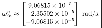
In degrees per hour,
Its magnitude is
Earth rotation has magnitude about 15.0411∘∕h. Therefore the transport rate in this fast-moving
example is of the same order as Earth rate. It cannot be neglected in a precise local-level
navigator.
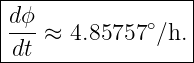
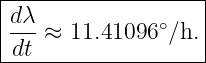
Solution 5: Geodetic position rates
The latitude rate is
Converting to degrees per hour,
The longitude rate is
or
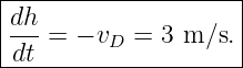
Finally,
The sign follows directly from the NED convention. Negative down velocity means climbing.
Solution 6: From inertial gyro rate to body rate relative to NED
At 45∘ latitude,
Adding the transport rate from Exercise 4,
For a level vehicle at heading 30∘,
The commanded body-relative yaw rate is
Therefore the ideal inertial gyro measurement is
or
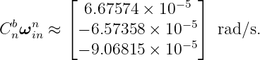
Now subtract the navigation-frame inertial rate in body coordinates:
The original 2∘∕s yaw rate relative to NED is recovered exactly.
Solution 7: DCM chain and round-trip consistency
At ϕ = 30∘, λ = 20∘,
For a level heading of 45∘,
The body-to-ECEF transformation is
which evaluates to
For vb = [100, 0, 0]T m/s,
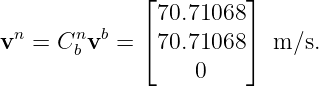
Directly in NED,
Transforming the ECEF result back gives
up to numerical roundoff.
Finally,
This single example checks matrix order, handedness, transpose convention, and norm
preservation.
Solution 8: Derivative consistency between ECEF and NED
The transport rate is the same as in Exercise 4,
Its cross product with velocity is
Rearrange the derivative relation:
Therefore
Using ϕ = 45∘ and λ = 30∘ gives
Substitute this result back:
The original NED derivative is recovered.
The extra cross-product term is essential because Cen is changing with time. Transforming the
ECEF coordinate derivative alone would compare derivatives taken in different rotating
bases.
Solution 9: Stationary Earth-fixed attitude consistency
At 60∘ latitude,
In degrees per hour this is
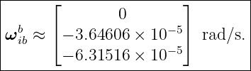
At heading 90∘,
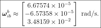
apart from tiny floating-point representations of cos 90∘. Thus the ideal gyro output
is
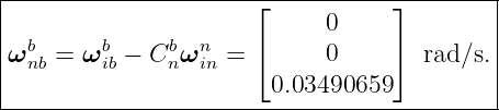
Since the body is fixed relative to NED,
The DCM equation gives
For this case both matrix terms evaluate numerically to
up to roundoff, so they cancel exactly:
This is an excellent unit test for a local-level attitude mechanization. A stationary Earth-fixed
IMU must not slowly rotate in the computed NED frame when Earth rate is modeled
correctly.
Solution 10: Why local NED becomes ill-conditioned near the poles
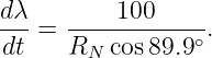
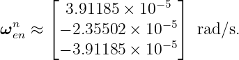
At ϕ = 89.9∘,
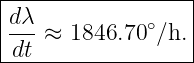
The longitude rate is
Numerically,
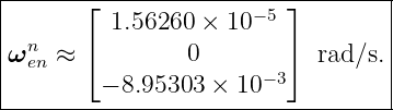
The transport rate is
In degrees per hour,
The large down-axis component comes from
which grows without bound as cos ϕ → 0 in the local longitude parameterization.
The vehicle is not physically rotating thousands of degrees per hour in inertial space. The singular
behavior comes from the local definition of North and longitude near the pole. An arbitrarily small
displacement near the pole can correspond to a very large change in longitude and a rapid rotation
of the local NED axes. This is why high-latitude inertial navigation often uses alternative local
frames, wander-azimuth frames, or ECEF mechanization instead of conventional NED coordinates
[1, 2].
3 What these examples establish
These calculations turn the frame hierarchy of INS06 into a set of concrete checks.
First, ECI, ECEF, NED, and body coordinates are representations of physical vectors, not different
physical vectors. Proper DCM transformations preserve vector magnitude and compose in a strict
order.
Second, a time derivative is more subtle than a coordinate transformation. When the destination
basis itself rotates, the derivative contains an angular-rate cross product. Exercise 8 is particularly
useful for testing this point in software.
Third, Earth rate and transport rate are reference-frame rates. They are not vehicle turn rates, but
they enter the attitude mechanization because the navigation frame itself rotates relative to
inertial space.
Fourth, position and velocity are coupled geometrically. North and east velocities rotate the
local frame and therefore change the reference rate that must be removed from gyro
measurements.
Finally, local NED coordinates have a geometric singularity near the poles. That singularity is a
property of the coordinate system, not a physical divergence of the vehicle dynamics.
4 Implementation checks suggested by this problem set
A strapdown implementation should reproduce at least the following numerical behaviors:
- Cen(C
en)T = I and det C
en = 1;
- vector norms are unchanged by ECEF/NED transformations;
- the round trip vn → ve → vn returns the original vector to numerical precision;
- ωenn = 0 for zero horizontal velocity;
- a stationary Earth-fixed IMU has ωnbb = 0, not ω
ibb = 0;
- the DCM derivative of a stationary Earth-fixed platform is zero after Earth-rate
subtraction;
- ECEF and NED vector derivatives agree only after the transport-rate derivative term
is included;
- the local NED longitude and transport-rate formulas should be guarded or replaced as
the poles are approached.
These are small calculations, but together they catch many of the frame-order, transpose, sign, and
reference-rate errors that otherwise appear later as unexplained attitude or position
drift.
References
[1] David H. Titterton and John L. Weston, Strapdown Inertial Navigation Technology,
2nd ed., Institution of Electrical Engineers, 2004.
[2] Paul D. Groves, Principles of GNSS, Inertial, and Multisensor Integrated Navigation
Systems, 2nd ed., Artech House, 2013.
[3] Christopher Jekeli, Inertial Navigation Systems with Geodetic Applications, Walter
de Gruyter, 2001.
[4] Paul G. Savage, “Strapdown Inertial Navigation Integration Algorithm Design Part
1: Attitude Algorithms,” Journal of Guidance, Control, and Dynamics, vol. 21, no. 1,
pp. 19–28, 1998.
[5] National Geospatial-Intelligence Agency, Department of Defense World Geodetic
System 1984: Its Definition and Relationships with Local Geodetic Systems,
NGA.STND.0036, Version 1.0.0, 2014.

![[parent]](https://images.physicslibrary.org/images/uparrow.png)


![[ ]
i 7000 0
r = 0 km.](https://images.physicslibrary.org/cache/objects/1355/make4ht/StrapdownInertialNavigationExamplesEarthRotationAndNavigationFrames6x.png)










![b [ ]T
v = 100 0 0 m ∕s](https://images.physicslibrary.org/cache/objects/1355/make4ht/StrapdownInertialNavigationExamplesEarthRotationAndNavigationFrames24x.png)





![n
dC-b-= Cn [ωb ]× − [ωn ]×Cn
dt b ib ie b](https://images.physicslibrary.org/cache/objects/1355/make4ht/StrapdownInertialNavigationExamplesEarthRotationAndNavigationFrames32x.png)




















![n
dC-b-= Cn [ωb ] − [ωn ] Cn .
dt b ib× ie × b](https://images.physicslibrary.org/cache/objects/1355/make4ht/StrapdownInertialNavigationExamplesEarthRotationAndNavigationFrames87x.png)