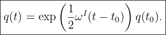
A quaternion describes orientation at an instant. Quaternion kinematics describes how that
orientation changes when a rigid body has angular velocity. This connection is fundamental in
inertial navigation, spacecraft attitude propagation, robotics, multibody dynamics, and simulation
because gyroscopes measure angular rate while an attitude estimator or controller usually needs an
orientation state.
The central result is simple but convention sensitive. For the PhysicsLibrary convention, angular
velocity resolved in the inertial frame multiplies the attitude quaternion on the left, while angular
velocity resolved in the body frame multiplies on the right.
1 Convention declaration and attitude meaning
This article uses the PhysicsLibrary quaternion convention:
right-handed orthonormal frames;
Hamilton multiplication, so ij = k;
scalar-first display notation,
(1)
the attitude quaternion is
(2)
which maps coordinates from the body frame B to the inertial or reference frame
I;
Scalar-last storage, such as [qx,qy,qz,qw]T, is also common in software. It changes only
the array layout, not the kinematic equations once the components have been mapped
correctly.
2 Angular velocity is one geometric vector
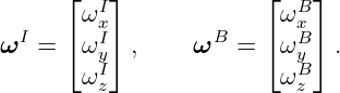
Let the physical angular velocity of the body relative to the inertial frame be ω. Its components
depend on the frame used to resolve it. Write
(4)
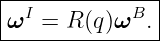
The two coordinate descriptions are related by the attitude matrix from Q09:
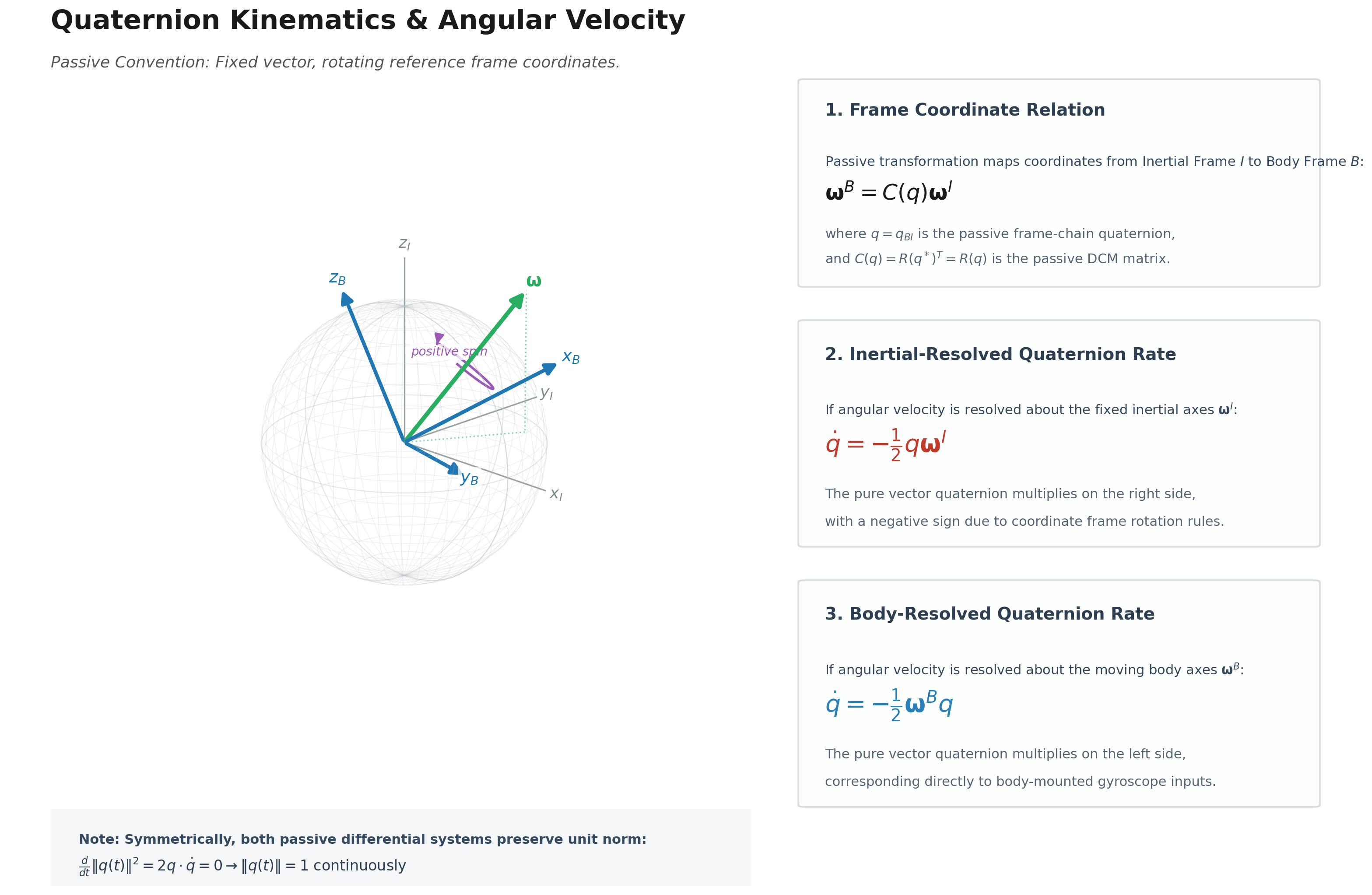
Figure 1 emphasizes that ωI and ωB are not two different physical angular velocities. They are
two coordinate descriptions of the same geometric vector.
Figure 1:Quaternion kinematics for the attitude q = IqB. The body frame is shown in blue,
the inertial frame in gray, and the physical angular velocity vector in green. The same angular
velocity may be resolved in either frame. Inertial resolved components multiply the attitude
quaternion on the left; body resolved components multiply it on the right.
3 Infinitesimal rotation over a short time
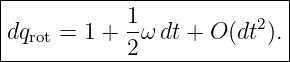
Over a short interval dt, a body rotating with angular speed∥ω∥ turns through the small physical
angle
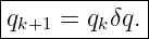
If the same infinitesimal physical rotation is resolved about inertial axes, it composes on the
left:
(15)
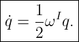
Therefore
(16)
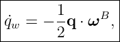
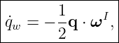
The scalar equation is unchanged,
(17)
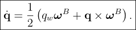
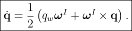
but the cross product order in the vector equation changes:
(18)
6 Why the two forms are equivalent
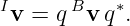
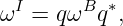
Since the pure angular velocity quaternions are related by the attitude rotation,
(19)
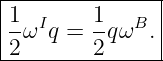
we have
(20)
for unit q. Hence
(21)
The two differential equations therefore describe exactly the same physical attitude motion. The
multiplication side changes only because the angular-rate components are expressed in different
frames.
7 Scalar-first matrix form
Define the scalar-first quaternion column
(22)
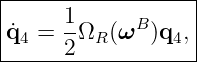
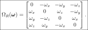
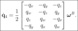
For body resolved angular velocity,
(23)
where
(24)
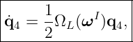
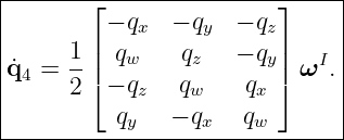
For inertial resolved angular velocity,
(25)
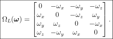
where
(26)
The different sign patterns encode left versus right quaternion multiplication.
8 Rate form driven directly by a three vector
The body rate equation can also be written as a 4 × 3 matrix multiplying the measured angular
rate vector:
(27)
For inertial resolved components,
(28)
These forms are convenient in estimation and simulation code because they map a measured three
component rate directly into a four component quaternion rate.
9 Norm preservation in continuous time
An exact attitude quaternion should remain unit length. Both rate matrices in equations (27) and
(29) are skew symmetric, so
(29)
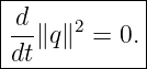
Therefore
(30)
Hence
(31)
The continuous differential equation preserves quaternion norm exactly. Any norm drift in a
numerical simulation is therefore a discretization effect, not a property of the exact
kinematics.
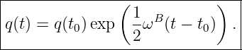
10 Constant angular velocity
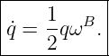
If ωB is constant in body coordinates, equation (13) has the exact solution
(32)
If ωI is constant in inertial coordinates,
(33)
For a nonzero angular rate vector, the exponential is
(34)
This is the exact finite quaternion increment for constant angular velocity over the
interval.
11 Gyroscope propagation
A body mounted gyroscope normally reports a sample of body resolved angular velocity. If the rate
is approximated as constant during a sample interval Δt, form
(35)
and update
(36)
This exact constant rate step is preferable to memorizing a sign pattern without first establishing
the frame and multiplication convention. Numerical integration methods and normalization
strategies are treated in Q13.
12 Checks that catch convention errors
Several simple cases are especially useful for implementation testing.
If ω = 0, then q = 0.
Starting from q = 1 with constant positive z-axis rate,
(37)
Replacing q by −q also replaces q by −q, so the physical attitude trajectory is
unchanged.
Body and inertial rate forms must agree after applying ωI = R(q)ωB.
The exact continuous rate equation must preserve ∥q∥ = 1.
13 Common pitfalls
The most common mistakes are:
using a body rate equation with inertial resolved angular velocity or the reverse;
putting angular velocity on the wrong multiplication side;
importing a kinematic equation from a source that defines the attitude quaternion in
the opposite frame direction;
confusing scalar-first and scalar-last memory layouts with different kinematic physics;
forgetting the factor of 1∕2, which follows from the quaternion half angle representation;
interpreting numerical norm drift as physical attitude behavior rather than integration
error.
14 What comes next
The next entry introduces relative attitude and error quaternions. Later, Q13 returns to
quaternion propagation and compares discrete numerical integration methods, exact exponential
updates, normalization, and sign continuity.
15 Sources and historical notes
Quaternion rate equations have long been used in spacecraft attitude systems. The 1977 NASA
Space Shuttle working relationships note by D. M. Henderson is a useful historical engineering
reference connecting Euler Angles, quaternions, and transformation matrices. Bach and Paielli’s
NASA Technical Memorandum 102798 develops quaternion attitude formulations in the context
of rigid-body state estimation and spacecraft control. The equations here are written
in the PhysicsLibrary convention rather than copied from either source, because the
multiplication side and signs depend on the precise frame and quaternion mapping
definitions.
References
[1]D. M. Henderson, Euler Angles, Quaternions, and Transformation Matrices Working
Relationships, NASA JSC-12960, July 1977.
[2]R. Bach and R. Paielli, Direct Inversion of Rigid-Body Rotational Dynamics, NASA
Technical Memorandum 102798, 1990.
License
This article is an original synthesis prepared for PhysicsLibrary and intended for release under CC
BY-SA 4.0.
"quaternion kinematics and angular velocity" is owned by bloftin.
This is version 4 of quaternion kinematics and angular velocity, born on 2026-08-24, modified 2026-08-27.
Object id is 1105, canonical name is QuaternionKinematicsAndAngularVelocity.
Accessed 336 times total.










![[ ]T
q4 = qw qx qy qz .](https://images.physicslibrary.org/cache/objects/1105/make4ht/QuaternionKinematicsAndAngularVelocity21x.png)