Laplace Transform: Why Transform a Differential Equation?

(Topic)

LT01: Why Transform a Differential Equation?

The Laplace transform is valuable because many physical problems are easiest to state in the time domain but easier to manipulate in a transform domain.

A typical model contains three ingredients:

a differential equation describing the dynamics,
initial conditions describing the state of the system at the starting time,
and an input or forcing function that may be smooth, discontinuous, delayed, or impulsive.

The central motivation for the Laplace transform is to reorganize these ingredients so that differentiation is replaced by algebraic multiplication while the initial conditions enter the algebra automatically.

The desired workflow is

time -domain IVP − → transform -domain algebra −→ time-domain solution.

(1)

This article develops why such a transformation would be useful before deriving the full transform machinery.

Figure 1. The goal of the Laplace-transform method is to move an initial-value problem into a domain where differentiation becomes algebraic, solve there, and then return to the time domain.

1 A differential equation is already an operator equation

Consider the first-order initial-value problem

dy- dt + ay = f(t), y(0) = y0.

(2)

The unknown is not one number. It is the entire function y(t).

The equation contains the derivative operator

d -- , dt

(3)

and asks for a function that satisfies both the differential relation and the initial condition.

Using the differential-operator symbol

D = d-, dt

(4)

Equation (2) may be written schematically as

(D + a )y = f.

(5)

This notation exposes an important idea. Solving the differential equation means, in some sense, undoing the operator D + a.

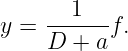
If D behaved like an ordinary number, we might be tempted to write

y = --1---f. D + a

(6)

That expression is only formal at this stage, but it points toward the motivation for transforms: find a representation in which the differentiation operator behaves more like multiplication by an ordinary variable.

2 Direct time-domain methods work, but each forcing can demand new work

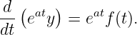
For Equation (2), the integrating-factor method is perfectly effective. Multiply by

eat.

(7)

Then

eatdy-+ aeaty = d- (eaty) , dt dt

(8)

d ( at ) at dt e y = e f (t).

(9)

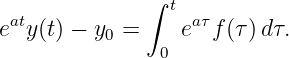
Integrating from 0 to t gives

∫ t eaty(t) − y0 = eaτf(τ) dτ. 0

(10)

Therefore

∫ t y(t) = e−aty0 + e− at eaτf(τ)d τ. 0

(11)

This is already a useful result. It separates the response into an initial-condition contribution and a forcing contribution.

But Equation (11) also reveals why a more systematic transform method is attractive. The details of the remaining integral depend on the form of f(t).

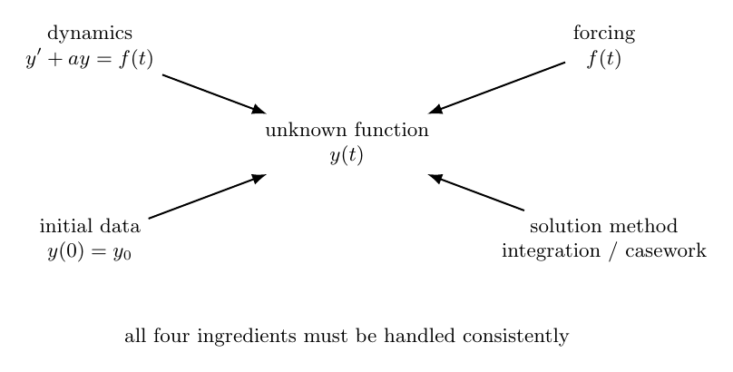
Figure 2. A time-domain initial-value problem combines dynamics, initial conditions, and forcing. Direct methods work, but the calculation can change substantially when the forcing changes.

3 The forcing function is often the awkward part

f (t) = 1,

(12)

the integral in Equation (11) is elementary.

f(t) = sinωt,

(13)

the integral requires a different calculation.

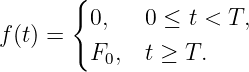
If the forcing turns on only after a delay T, then a piecewise definition may be needed:

{ 0, 0 ≤ t < T, f (t) = F0, t ≥ T.

(14)

If the forcing changes several times, the bookkeeping grows.

If the input is impulsive, the ordinary time-domain description requires the Dirac delta distribution.

Thus the difficulty is often not that one particular differential equation is impossible to solve. The difficulty is that many different forcing functions require repeated case-by-case manipulations.

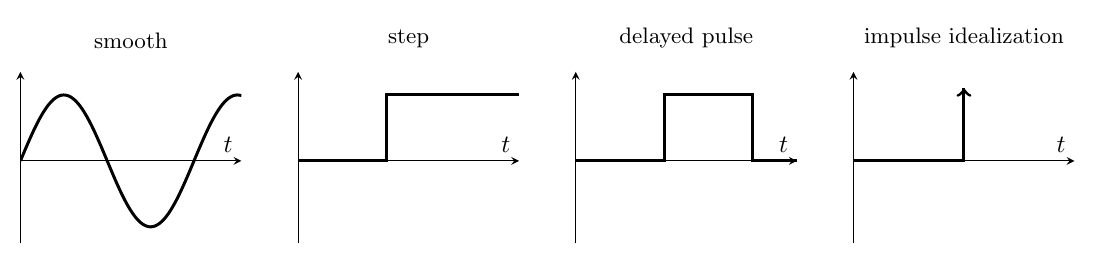
Figure 3. Linear systems may be driven by smooth, step-like, delayed, or impulsive inputs. A useful transform method should handle all of them within one consistent framework.

4 What would an ideal transform do?

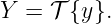
Suppose there were an operation 𝒯 that maps a time-domain function y(t) to a new representation Y :

Y = 𝒯 {y}.

(15)

For differential equations, we would like this operation to have several properties.

Linearity

h (t) = αf (t) + βg (t),

(16)

we would like

𝒯 {h} = α 𝒯 {f} + β𝒯 {g }.

(17)

This preserves the linear structure of the differential equation.

Differentiation should become algebraic

Instead of carrying the derivative operator D into the transformed problem, we would like something resembling

D −→ multiplication by a transform variable.

(18)

The Laplace transform will accomplish this in a slightly richer form because initial conditions also appear.

Initial conditions should enter naturally

A method for initial-value problems should not require us to solve the transformed equation first and then reconstruct the initial constants later.

The Laplace transform will encode initial data directly into the transformed derivative formulas.

Common inputs should have reusable transformed forms

If a step, exponential, sine wave, delay, or impulse appears repeatedly in engineering and physics, we would like to transform it once and reuse the result.

These requirements explain the structure of the LT series that follows.

5 Preview: how differentiation becomes algebra

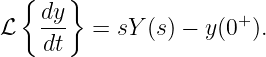
The key derivative identity will later be derived from the Laplace integral using integration by parts. For now, preview the result:

{ } dy- + ℒ dt = sY (s) − y (0 ).

(19)

The derivative has been replaced by multiplication by s, plus a term containing the initial value.

For the second derivative,

{ d2y} ℒ --2- = s2Y (s) − sy (0+) − y′(0+ ). dt

(20)

The pattern is exactly what we hoped for: Powers of the differentiation operator become powers of an algebraic variable.

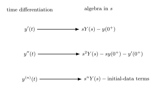
Figure 4. The central operational benefit of the Laplace transform. Time differentiation becomes multiplication by powers of s, while initial-condition terms appear explicitly. LT13 and LT14 will derive these formulas from first principles.

6 A first-order transform preview

Return to

′ y + ay = f(t), y (0 ) = y0.

(21)

Let

Y (s) = ℒ{y (t)}, F (s) = ℒ{f (t)}.

(22)

Using linearity and the preview identity in Equation (19), the transformed equation becomes

[sY (s) − y0] + aY (s) = F(s).

(23)

Collect the terms containing Y (s):

(s + a)Y (s) = F (s) + y0.

(24)

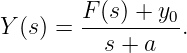
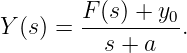
Now solve algebraically:

F-(s)-+-y0 Y(s) = s + a .

(25)

Compare this with the original differential equation. The transformed problem contains no time derivative of the unknown function. The differential equation has become an algebraic equation for the transformed unknown Y (s).

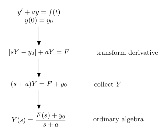
Figure 5. Preview of the first-order Laplace workflow. The derivative and initial value are absorbed into an algebraic equation for Y (s). Later articles will derive the transform pairs and inverse-transform steps needed to complete the solution.

7 Why the initial condition appearing automatically matters

In a direct time-domain solution, the homogeneous solution is often found first:

−at yh(t) = Ce .

(26)

The constant C is then determined from the initial condition.

The Laplace method reorganizes this process. The initial value y₀ enters Equation (25) immediately through the transformed derivative.

This is particularly useful for higher-order equations, where several initial conditions may appear:

y (0 ), y′(0 ), y′′(0), ...

(27)

The transform-domain equation carries these values explicitly rather than hiding them inside unknown integration constants.

8 The same idea scales to second-order dynamics

Consider the mass-spring-damper system

m ¨x + c˙x + kx = F (t),

(28)

with

x (0 ) = x0, x˙(0) = v0.

(29)

The transformed derivative previews are

ℒ{ ˙x} = sX (s) − x , 0

(30)

and

2 ℒ {¨x} = s X (s) − sx0 − v0.

(31)

Applying them to Equation (28) gives

	m + c + kX(s)
	= F(s).	(32)

Collecting the unknown transform,

( ) ms2 + cs + k X (s) = F (s) + m (sx0 + v0) + cx0.

(33)

Therefore

F-(s)-+-m-(sx0-+-v0) +-cx0- X (s) = ms2 + cs + k .

(34)

The differential operator

2 mD + cD + k

(35)

has become the polynomial

2 ms + cs + k.

(36)

This is one of the most important structural changes produced by the transform.

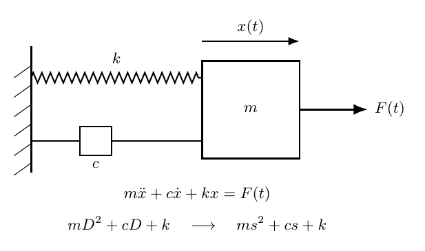
Figure 6. Canonical second-order mechanical system. The Laplace transform converts the mass, damping, and stiffness differential operator into the polynomial ms² + cs + k.

9 Why algebraic denominators are useful

The denominator

ms2 + cs + k

(37)

contains important information about the dynamics.

Its roots are related to the natural modes of the system. Later, when the complex s-plane is introduced, those roots will become poles of the transformed response.

The same denominator appears for many different inputs F(t). This means the system dynamics can be separated conceptually from the particular forcing.

For zero initial conditions, Equation (34) reduces to

X (s) = -----1-------F(s). ms2 + cs + k

(38)

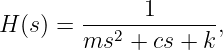
This suggests defining a system function

------1------ H (s) = ms2 + cs + k ,

(39)

so that

X (s) = H (s)F (s).

(40)

LT27 will develop this idea as the transfer-function description of a linear system.

10 The system viewpoint

A linear system can be viewed as a map from an input to an output:

input −→ system −→ output.

(41)

In the time domain, this relationship may involve a differential equation or convolution integral.

In the Laplace domain, zero-state linear time-invariant systems often reduce to multiplication:

Y (s ) = H (s)U (s).

(42)

This is a major simplification. A complicated time-domain operation becomes an algebraic product.

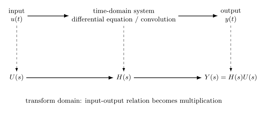
Figure 7. The system viewpoint. In the time domain the input-output relation may require a differential equation or convolution. In the Laplace domain a zero-state linear time-invariant system is represented algebraically by multiplication with H(s).

11 Discontinuous forcing is where the method becomes especially attractive

Suppose a force is applied at time T rather than at t = 0. In the time domain this naturally creates piecewise definitions.

Laplace-transform methods introduce systematic representations for such inputs using the Heaviside step function. Delays become algebraic exponential factors in the transform domain.

Similarly, impulse inputs can be represented using the Dirac delta function and handled within the same transform framework.

The important point at LT01 is not yet the detailed formulas. It is that one transform language can handle

ordinary smooth forcing,
sudden switching,
delayed inputs,
piecewise forcing,
and impulsive inputs.

This uniformity is one reason the method became so important in engineering, control, circuits, and mathematical physics.

12 What the Laplace transform does not eliminate

The transform does not make every problem trivial.

Several tasks remain:

the transform of the forcing must be found,
the transformed algebraic expression may need factorization or partial fractions,
the inverse transform must be computed,
convergence conditions must be respected,
and nonlinear differential equations generally do not become simple algebraic equations in the same way.

The method is especially powerful for linear initial-value problems because linearity, differentiation, and common forcing functions fit the transform structure naturally.

13 A comparison of the direct and transform viewpoints

For a first-order linear equation, the direct method emphasizes integration:

∫ −at − at t aτ y(t) = e y0 + e e f(τ)d τ. 0

(43)

The transform method emphasizes algebra:

F (s) + y0 Y(s) = ----------. s + a

(44)

These are not competing truths. They are two representations of the same dynamics.

The direct solution makes the time-domain accumulation explicit. The transform solution packages that accumulation into algebraic structure that can be manipulated systematically.

Later, the convolution theorem will show exactly how these two viewpoints are connected.

14 The core conceptual payoff

The main reason to transform a differential equation can now be stated precisely.

A transform is useful when it changes the representation of a problem so that difficult operations become simpler ones.

For the Laplace transform, the central simplifications are

differentiation becomes multiplication by powers of s plus explicit initial-condition terms,
linear differential equations become algebraic equations,
common forcing functions acquire reusable transform representations,
delayed and impulsive inputs can be handled systematically,
convolution becomes multiplication,
and the system dynamics can be separated from the particular input through a transfer function.

This is why the Laplace transform is more than a table of integrals. It is a change of mathematical representation designed to match the structure of linear dynamical systems.

15 What comes next: why exponentials are the natural functions

LT01 has previewed the operational benefit

D −→ s.

(45)

The next question is deeper:

Why should an exponential kernel be the mechanism that produces this simplification?

LT02 answers that question by studying exponential functions as eigenfunctions of differentiation.

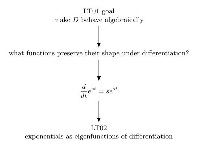
Figure 8. LT01 establishes the desired operational effect: replace time differentiation by algebra. LT02 explains why exponential functions are the natural functions for accomplishing that transformation.

16 Self-check questions

What three ingredients usually define an initial-value problem?
Why can changing the forcing function make a direct time-domain calculation more cumbersome?
What property would an ideal transform have with respect to differentiation?
Why is the appearance of initial conditions in the transformed derivative formula useful?
What does the first-order equation y′ + ay = f(t) become algebraically after the derivative transform is applied?
What polynomial replaces the mass-spring-damper operator mD² + cD + k?
Why is the same transformed denominator useful for many different inputs?
What is meant by separating system dynamics from forcing?
Why are delayed and impulsive inputs strong motivations for the Laplace method?
What important mathematical work still remains after a differential equation has been transformed?

17 Summary

A differential equation is difficult because the unknown function appears under differential operators and must also satisfy initial conditions and forcing constraints.

The Laplace transform is designed to reorganize the problem so that

d --− → s dt

(46)

in an algebraic sense, while initial conditions appear explicitly.

The first-order equation

y′ + ay = f(t)

(47)

is previewed as

(s + a)Y (s) = F (s) + y , 0

(48)

and the second-order equation

m ¨x + cx˙+ kx = F(t)

(49)

becomes an equation involving the polynomial

ms2 + cs + k.

(50)

The next step is to understand why exponentials are naturally connected to this replacement of differential operators by algebraic factors.

References

[1] E. Kreyszig, Advanced Engineering Mathematics, Wiley.

[2] R. V. Churchill, Operational Mathematics, McGraw-Hill.

[3] G. Doetsch, Introduction to the Theory and Application of the Laplace Transformation, Springer.

"Laplace Transform: Why Transform a Differential Equation?" is owned by bloftin.
(view preamble)