Gravitational Fields, Superposition, and Continuous Mass Distributions
M07-01 described gravity as a force between masses.
The gravitational-field viewpoint separates the source of gravity from the test object used to probe
it.
At a position
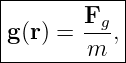
define The Gravitational Field by
where
is a test mass placed at that point.
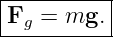
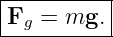
Thus the gravitational force on a test mass is
The field is a property of the source masses and their arrangement.
It does not depend on the mass of the test object when gravitational and inertial mass are
identified in the Newtonian model.
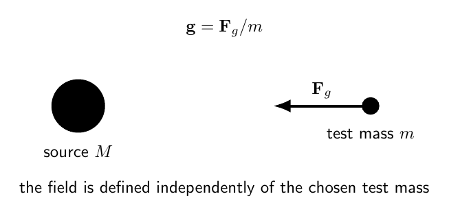
Figure 1. Source masses create a gravitational field in the surrounding space. A test mass placed
at a point experiences force Fg = mg.
1 Units and dimensions of the gravitational field
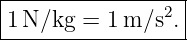
Because
the SI units are
Using
we obtain
Thus gravitational field and gravitational acceleration have the same dimensions.
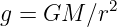
For a freely falling test object,
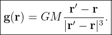
2 Field of a single point mass
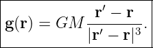
Place a source mass
at position
A test mass
at
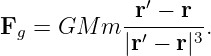
experiences
Divide by
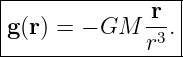
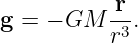
If the source is at the origin,
then
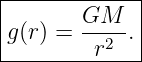
The magnitude is
The direction is radially inward.
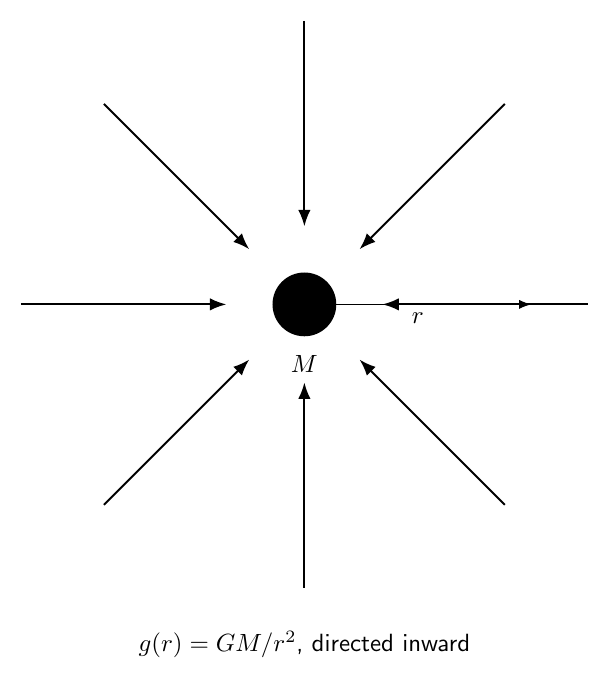
Figure 2. The gravitational field of a point mass is radial, inward, and inverse square in
magnitude. The field is undefined at the idealized point source itself.
3 Field versus force
The distinction is important.
The field
is created by the source masses.
The force
depends additionally on the test mass:
If the test mass doubles:
- the gravitational field at that location is unchanged,
- the gravitational force doubles.
4 Example 1: field of a small source mass
Let
and
Then
| g | =  | (25)
|
| = 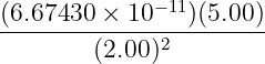 | (26)
|
| = 8.34 × 10⁻¹¹ m∕s2. | (27) |
A
test mass at that point would experience force magnitude
5 Superposition of gravitational fields
Newtonian gravity is linear in the source masses.
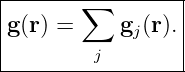
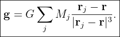
If several point masses are present, the total field is the vector sum of the individual
fields:
For point masses
at positions
Once
is known, the force on any test mass is
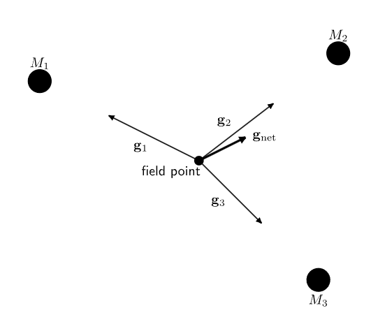
Figure 3. Gravitational fields obey vector superposition. The net field is the vector sum of the
fields produced by all source masses.
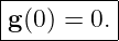
6 Example 2: two equal masses at a midpoint
Let equal source masses
be placed at
and
At the origin, the field from the right mass points in the
direction.
The field from the left mass points in the
direction.
The magnitudes are equal:
Therefore
This is cancellation by symmetry.
The field is zero at the midpoint even though each source produces a nonzero field there.
7 Example 3: unequal collinear masses
Place
at
and
at
At a point between them,
the fields point in opposite directions.
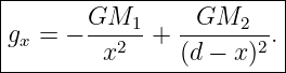
Taking
to the right,
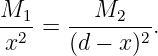
A zero-field point satisfies
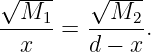
Taking positive square roots,
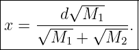
Solving,
The balance point lies closer to the smaller mass.
8 From discrete masses to continuous matter
Real objects contain enormous numbers of particles.
Instead of summing individual masses, we replace the sum by an integral.
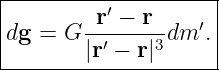
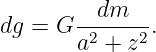
An infinitesimal source mass
at
produces
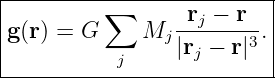
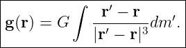
Therefore
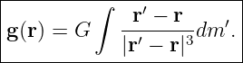
This is the basic gravitational-field integral for a continuous mass distribution.
9 Line mass density
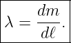
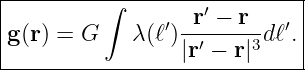
For a thin wire or rod, define line mass density
Its units are
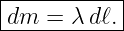
Then
If the density varies along the object,
10 Surface mass density
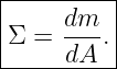
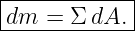
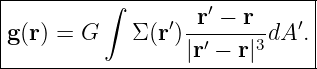
For a thin sheet, disk, or shell, define surface mass density
Its units are
Then
11 Volume mass density
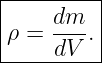
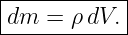
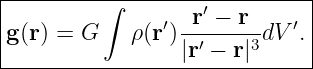
For a three-dimensional body, define volume mass density
Its units are
Then
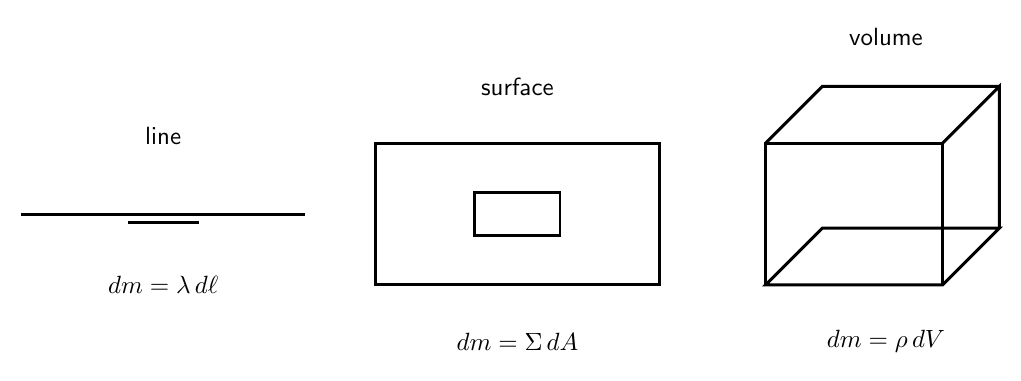
Figure 4. Continuous mass models use line density λ, surface density Σ, or volume density ρ
according to whether the source is idealized as one-, two-, or three-dimensional.
12 The three common gravitational integrals
For a line distribution,
For a surface distribution,
For a volume distribution,
The structure is always the same.
The only change is the mass element.
13 A reliable setup procedure
For continuous gravitational-field problems:
- Choose coordinates that match the geometry.
- Identify the observation point.
- Write the source position r′.
- Write the vector from observation point to source element.
- Write dm′ using the correct density.
- Form dg.
- Use symmetry before integrating.
- Integrate only the components that survive.
- Check units and limiting cases.
Symmetry often removes most of the vector algebra.
14 Symmetry before calculus
Suppose a mass distribution is symmetric about an axis.
At a point on that axis, source elements related by rotation produce transverse field components
that cancel.
Only the axial component survives.
Similarly, for a distribution symmetric about a plane, some field components cancel in
pairs.
Using symmetry first can turn a difficult vector integral into one scalar integral.
15 Field on the axis of a uniform ring
Consider a thin ring of:
- radius a,
- total mass M,
- center at the origin,
- plane in the xy plane.
Find the field at
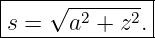
Every ring element lies the same distance from the observation point:
By rotational symmetry, all transverse components cancel.
Only the
component survives.
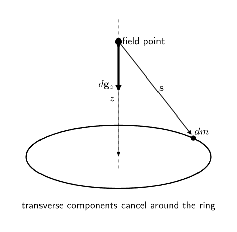
Figure 5. For a point on the symmetry axis of a uniform ring, transverse field components cancel
in pairs and only the axial component survives.
16 Derivation of the ring field
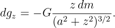
For a mass element
the field magnitude is
The axial projection factor is
For
the field points toward the ring plane, so
The geometric factor is constant around the ring.
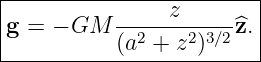
Therefore
| gz | = −G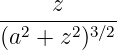 ∫
dm | (78)
|
| = −GM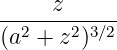 . | (79) |
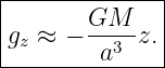
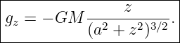
Thus
17 Checks on the ring result
At the center,
so
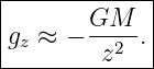
Far from the ring,
Then
and
The ring looks like a point mass from far away.
Near the center along the axis,
Then
so
Along the symmetry axis, the field is approximately linear near the center.
18 Example 4: numerical ring field
Let
and
Then
| |gz| | = GM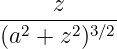 | (92)
|
| ≈ 5.97 × 10⁻⁹ m∕s2. | (93) |
The direction is toward the ring plane.
19 Field of a finite uniform rod on its perpendicular bisector
Consider a uniform rod:
- extending from x = −a to x = +a,
- lying on the x axis,
- line density λ.
Find the field at
A source element at
has mass
The distance to the observation point is
By left-right symmetry, horizontal components cancel.
Only the vertical component remains.
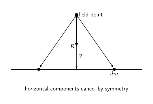
Figure 6. On the perpendicular bisector of a uniform rod, horizontal field components cancel by
symmetry and only the component directed toward the rod survives.
20 Derivation of the rod field
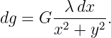
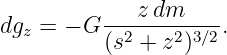
The field element magnitude is
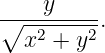
The vertical projection factor is
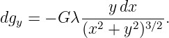
Thus
Integrate:
| gy | = −Gλy ∫
−aa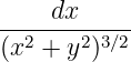 | (101)
|
| = −Gλy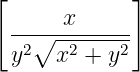 −aa. | (102) |
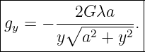
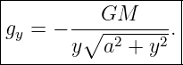
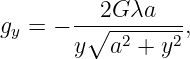
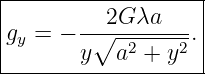
Therefore
Since
this can also be written
21 Far-field check for the rod
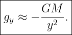
If
then
Therefore
Again, a localized extended body looks like a point mass from sufficiently far away.
22 Infinite-line limit
Hold
fixed and let
From
we obtain
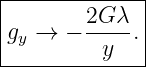
An infinite line produces a
field rather than an inverse-square field.
The geometry of the source changes how the field spreads.
23 Field on the axis of a uniform disk
Consider a thin disk:
- radius R,
- uniform surface density Σ,
- lying in the xy plane.
Find the field at
Build the disk from concentric rings.
A ring of radius
and width
has area
Its mass is
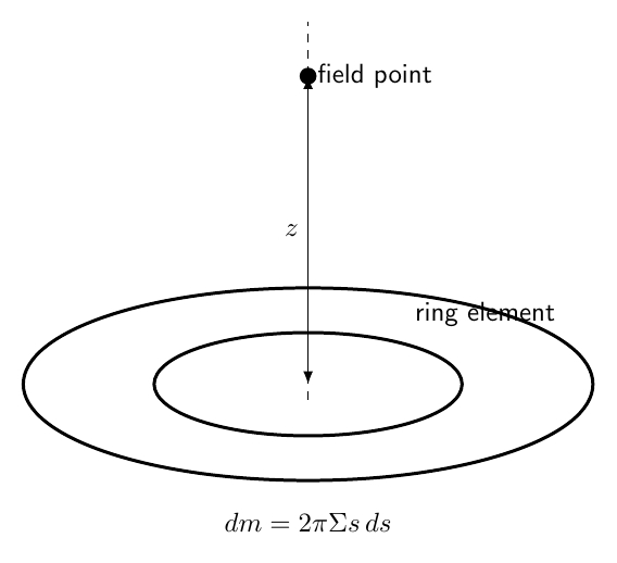
Figure 7. A uniform disk can be decomposed into concentric rings. Each ring contributes only an
axial field component at a point on the symmetry axis.
24 Derivation of the disk field
Using the ring result,
Substitute
Integrate from
to
| gz | = −2πGΣz ∫
0R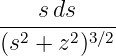 | (124)
|
| = −2πGΣz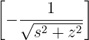 0R. | (125) |
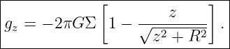
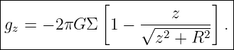
For
The direction is toward the disk.
25 Infinite-sheet limit
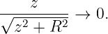
Let
Then
Thus
The field of an infinite uniform sheet is independent of distance from the sheet.
This differs strikingly from:
- point mass: g ∝ 1∕r2,
- infinite line: g ∝ 1∕r,
- infinite sheet: constant g.
26 Far-field check for the disk
For
expand
Then
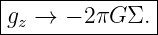
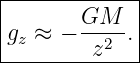
| gz | ≈−2πGΣ | (133)
|
| = − . | (134) |
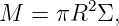
Since
The finite disk also approaches point-mass behavior in the far field.
27 Example 5: numerical disk field
Let
and
Then
| |gz| | = 2πGΣ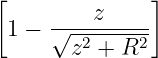 | (140)
|
| ≈ 1.16 × 10⁻⁹ m∕s2. | (141) |
28 Why source dimension changes distance scaling
The field of one isolated point source spreads through three-dimensional space.
Its magnitude decreases as
An infinite line has translational symmetry along one direction.
The remaining transverse spreading gives
An infinite sheet has translational symmetry in two directions.
Its field does not weaken with perpendicular distance.
These results can be understood geometrically even before introducing Gauss’s Law for
gravity.
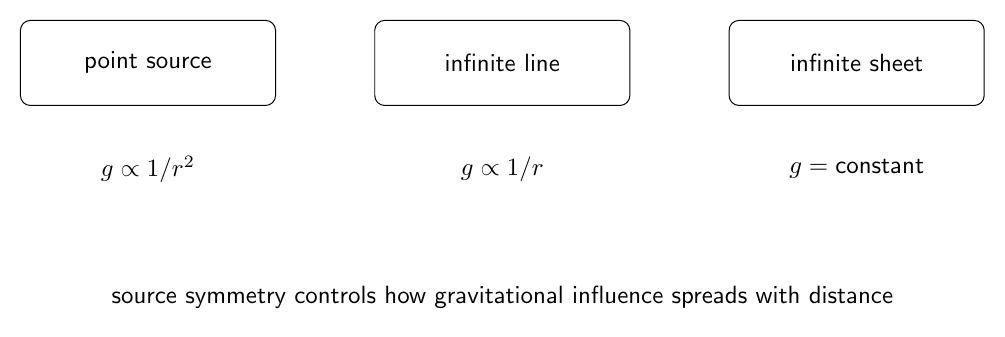
Figure 8. Source geometry strongly affects distance scaling: point-like sources give inverse-square
behavior, an infinite line gives inverse-distance behavior, and an infinite sheet gives a constant
field magnitude.
29 Far-field point-mass behavior
For any localized mass distribution with total mass
the leading far-field behavior is typically
when
is much larger than the source size.
The detailed shape of the source enters through smaller corrections.
A systematic treatment of those corrections leads to multipole expansions, which belong later in
the gravitation sequence.
30 Field at symmetry points
Symmetry can make the field vanish.
Examples include:
- the center of a uniform ring,
- the midpoint between two equal point masses,
- the center of many symmetric mass configurations.
A zero field does not imply a zero gravitational environment.
Nearby points may experience nonzero fields.
The spatial variation of the field determines tidal effects.
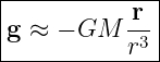
31 The field of a spherical body
A spherically symmetric body requires special treatment.
Outside such a body, the field turns out to be exactly the same as that of a point mass containing
the same total mass:
Inside a spherical shell, the net gravitational field vanishes.
These are Newton’s shell theorems.
They are important enough to deserve a separate derivation.
M07-03 develops those results from geometry and superposition.
32 Field singularities and idealizations
The point-mass field
diverges as
This singularity is a consequence of the point-particle idealization.
Real extended bodies have finite size and a distributed density.
Their fields must be computed using the actual mass distribution when the observation point lies
within or very near the body.
Similarly:
- an infinitely thin line,
- an infinitely thin sheet,
- an infinite spatial extent
are ideal mathematical models.
They are useful when the physical geometry is well approximated by those limits.
33 Gravitational field lines
A gravitational field line is drawn so that its tangent points in the direction of
For positive mass in Newtonian gravity:
- field lines point toward mass,
- field-line density can be used qualitatively to indicate field strength,
- field lines do not represent physical strings or trajectories.
A freely falling particle initially at rest begins accelerating tangent to the local field, but its later
path need not remain on one field line because of inertia.
34 Common mistakes
- Confusing gravitational field with gravitational force.
- Multiplying by the test mass when only the field is requested.
- Forgetting that the field points toward positive source mass.
- Adding field magnitudes instead of vectors.
- Using 1∕r2 with the wrong separation vector.
- Forgetting that a zero field at a symmetry point can result from cancellation.
- Mixing line, surface, and volume density units.
- Writing dm = ρdA or dm = Σ dV .
- Integrating vector components that symmetry guarantees will cancel.
- Forgetting the projection factor in ring, rod, or disk problems.
- Applying point-mass behavior at distances comparable to the source size without
justification.
- Counting the fixed geometry incorrectly when taking an infinite-line or infinite-sheet
limit.
- Assuming every extended source retains an inverse-square dependence at all distances.
- Applying the spherical point-mass result before establishing the shell theorem.
- Treating ideal singularities as literal predictions for finite physical matter.
35 Practice exercises
- Derive the point-mass field from Newton’s gravitational-force law.
- Show that N∕kg is equivalent to m∕s2.
- Reproduce Example 1 for a 5 kg source mass at 2 m.
- For two equal point masses, prove that the field vanishes at the midpoint.
- Derive the zero-field location between two unequal collinear point masses.
- Write the gravitational-field integral for line, surface, and volume densities.
- Derive the field on the symmetry axis of a uniform ring.
- Show that the ring field approaches point-mass behavior for |z|≫ a.
- Show that the ring field is linear in z near the center along the symmetry axis.
- Derive the field on the perpendicular bisector of a finite uniform rod.
- Take the infinite-line limit of the finite-rod result.
- Derive the on-axis field of a uniform disk by integrating rings.
- Take the infinite-sheet limit of the disk result.
- Show that a finite disk approaches point-mass behavior in the far field.
- Explain geometrically why point, infinite-line, and infinite-sheet sources have different
distance scalings.
36 Summary
The gravitational field is
A point source mass
at
produces
For several point masses,
For continuous matter,
The mass element is chosen according to geometry:
A uniform ring produces the axial field
A finite rod of half-length
on its perpendicular bisector produces
A uniform disk produces
Superposition and symmetry are the main tools for gravitational fields of extended
matter.
References
References
[1] PhysicsLibrary, M07-01, Newton’s Law of Universal Gravitation.
[2] J. R. Taylor, Classical Mechanics, University Science Books, 2005.
[3] D. Kleppner and R. Kolenkow, An Introduction to Mechanics, 2nd ed., Cambridge
University Press, 2014.
[4] J. B. Marion and S. T. Thornton, Classical Dynamics of Particles and Systems, 5th
ed., Brooks/Cole, 2004.