|
|
|
|||||||
and
Use
Unless otherwise stated, gains and losses used in cascade formulas are power ratios in linear units.
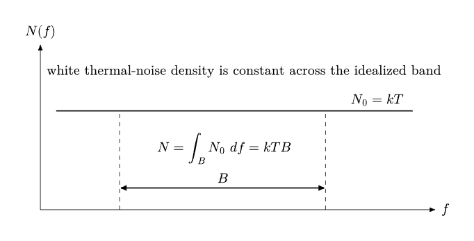
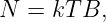
Figure. White thermal-noise density integrates over receiver bandwidth. The density is N0 = kT, while the total available noise power is N = kTB.
Part I: Exercises
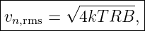
Exercise 1: Johnson noise voltage and matched noise powerA 50.0 Ω resistor is at 290 K and is observed over a 1.00 MHz bandwidth. Find (a) the RMS open-circuit Johnson-noise voltage, (b) the available noise power delivered to a matched load, and (c) that noise power in dBm. Verify that the matched power is independent of the resistance value.
Exercise 2: thermal-noise power in a receiver bandwidthAt 290 K, calculate the available thermal-noise power in a 2.00 MHz bandwidth. Express the result in watts, dBW, and dBm. Compare it with the familiar −174 dBm/Hz room-temperature noise density.
Exercise 3: noise density at a colder temperatureFind N0 = kT at T = 150 K in (a) W/Hz, (b) dBW/Hz, and (c) dBm/Hz. By how many decibels is this below the 290 K noise density?
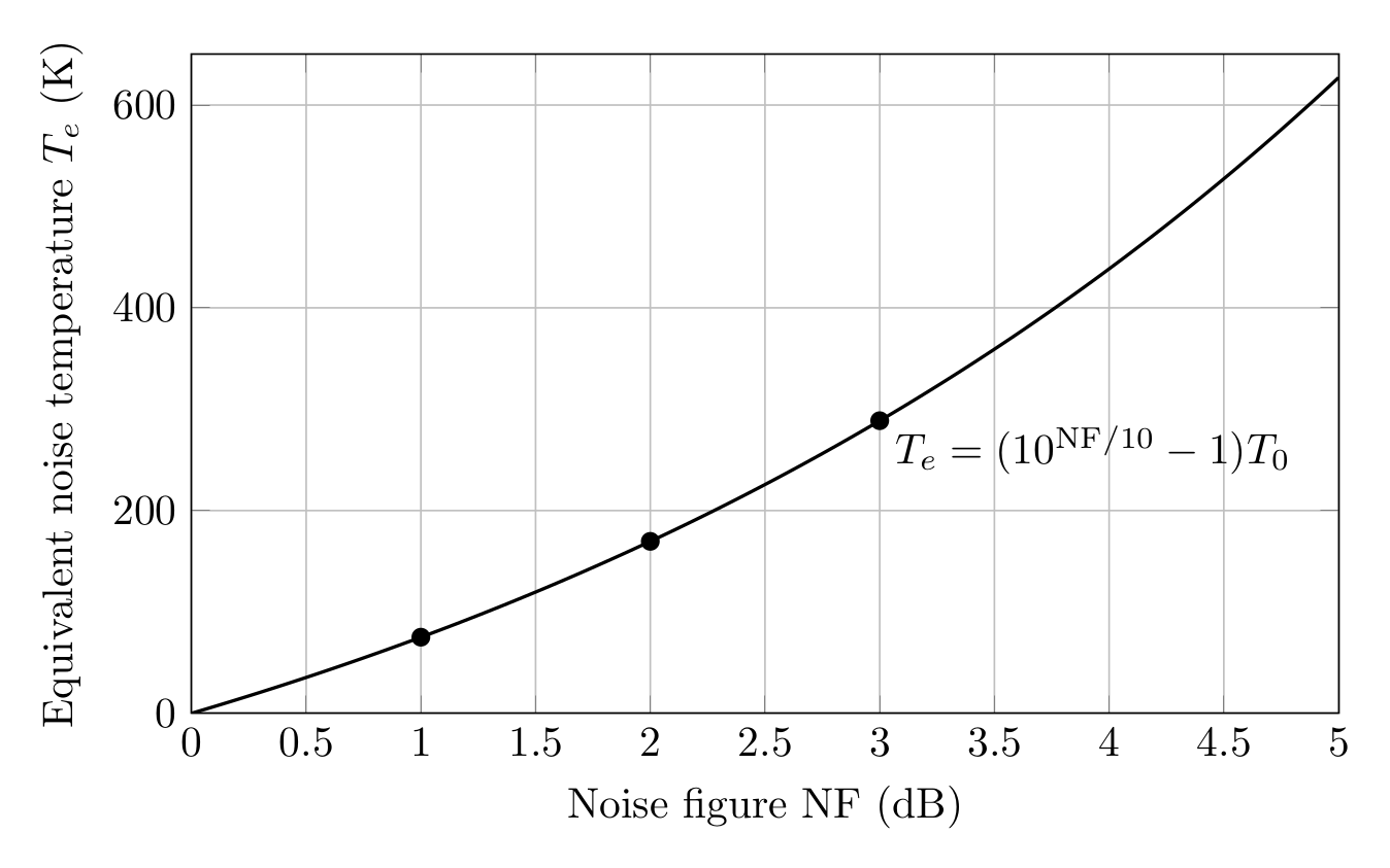
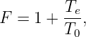
Figure. Equivalent input noise temperature increases nonlinearly with noise figure. The conversion uses Te = (10NF∕10 − 1)T 0.
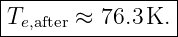
Exercise 4: noise figure to equivalent noise temperatureAn amplifier has noise figure NF = 1.20 dB. Find its linear noise factor F and equivalent input noise temperature Te referred to T0 = 290 K.
Exercise 5: equivalent noise temperature to noise figureA receiver front end has equivalent input noise temperature Te = 80.0 K. Find its noise factor and noise figure.
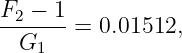
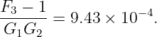
Exercise 6: three-stage cascaded receiverA three-stage receiver has
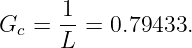
Calculate the total input-referred noise factor, total noise figure, and total equivalent input noise temperature. Quantify how strongly the first-stage gain suppresses stages 2 and 3.
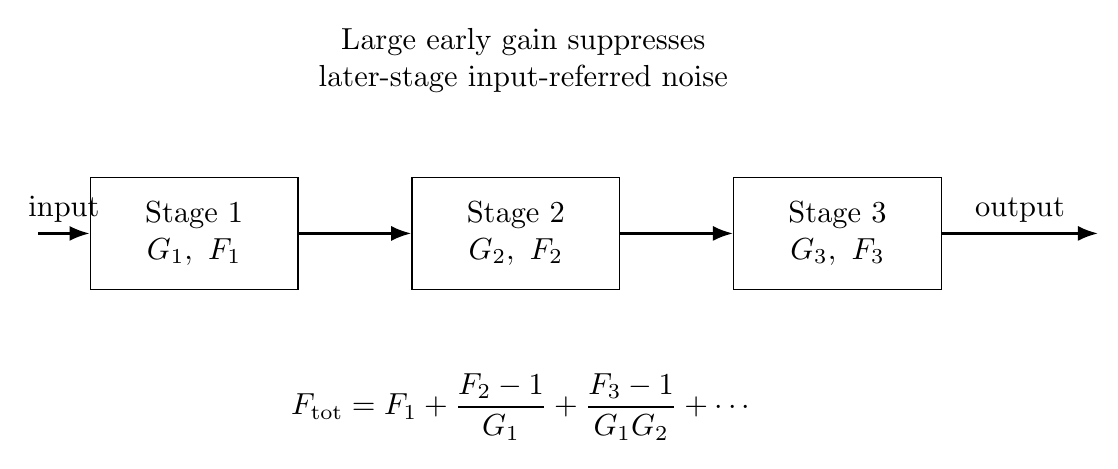
Figure. Friis cascade noise formula. High gain in the first low-noise stage reduces the input-referred importance of later-stage noise.
Exercise 7: why loss before an LNA is expensiveA cable has 1.50 dB power loss at 290 K. An LNA has 1.00 dB noise figure and 20.0 dB gain. Compare two cases: (a) cable before LNA and (b) cable after LNA. Find the total cascade noise figure and equivalent input noise temperature in both cases.
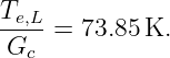
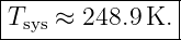
Exercise 8: antenna temperature and system noise temperatureAn antenna has noise temperature TA = 120 K and a receiver referred to the same input plane has equivalent noise temperature Te,rx = 80.0 K. Find (a) Tsys, (b) N0 in W/Hz, and (c) N0 in dBW/Hz and dBm/Hz.
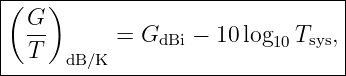
Exercise 9: receiver figure of merit G∕TA receiving antenna has directional gain 28.0 dBi and the complete receiver system has Tsys = 150 K at the same reference plane. Calculate G∕T in dB/K. Explain what physical change would improve G∕T by 3 dB.
Exercise 10: C∕N0 from carrier power and system temperatureAt the receiver reference plane, the carrier power is C = −155 dBW and Tsys = 250 K. Calculate the noise density in dBW/Hz and the resulting C∕N0 in dB-Hz.
Exercise 11: direct C∕N0 link budget using G∕TAn illustrative RF link has
Use the direct link-budget form to find C∕N0. Use −10 log 10k ≈ 228.60 dB-K/Hz.
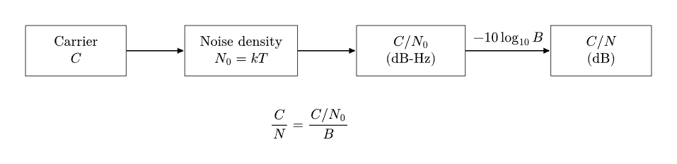
Figure. C∕N0 compares carrier power with noise density. Choosing a bandwidth integrates that density and converts the result to C∕N.
Exercise 12: converting C∕N0 to C∕NA receiver measures C∕N0 = 45.0 dB-Hz. What is C∕N in a noise-equivalent bandwidth of 2.00 MHz?
Exercise 13: infer receiver bandwidth from C∕N0 and C∕NA receiver has C∕N0 = 48.0 dB-Hz and measured C∕N = 8.00 dB. Assuming thermal noise dominates and the stated bandwidth is a noise-equivalent bandwidth, determine B.
Exercise 14: bandwidth penaltyA fixed carrier has C∕N0 = 50.0 dB-Hz. Compute C∕N for bandwidths of 10.0 kHz and 20.0 kHz. Show explicitly that doubling bandwidth degrades C∕N by approximately 3.01 dB.
Exercise 15: GNSS-style weak-signal exampleAn illustrative GNSS-like receiver has carrier power C = −158.5 dBW and system noise temperature Tsys = 400 K. Find (a) N0 in dBW/Hz, (b) C∕N0 in dB-Hz, and (c) C∕N in a 2.00 MHz front-end noise bandwidth. Interpret how C∕N can be negative while C∕N0 remains a useful receiver-quality metric.
Exercise 16: reference-plane bookkeeping with feed loss and an LNAAt the antenna terminals, TA = 100 K. A 1.00 dB feed loss at 290 K precedes an LNA having NF = 0.80 dB and 25.0 dB gain. Refer all noise to the antenna-terminal plane. Find (a) the feed equivalent noise temperature, (b) the LNA equivalent input noise temperature, (c) total system noise temperature, and (d) G∕T if the receive antenna gain is 25.0 dBi. If the carrier at the same antenna-terminal reference plane is C = −160 dBW, also find C∕N0.
Part II: Complete Worked Solutions
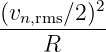
Solution 1: Johnson noise voltage and matched noise powerThe open-circuit mean-square voltage is
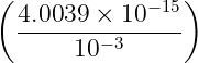
Therefore
Thus
With a matched load, only half the open-circuit voltage appears across the load. The delivered power is
Hence
In dBm,
Therefore
The resistance cancels algebraically. Changing R changes the noise voltage, but a matched resistor at the same temperature and bandwidth has the same available noise power kTB.
Solution 2: thermal-noise power in a receiver bandwidthUsing
we obtain
Thus
The logarithmic values are
At 290 K the density is approximately −173.98 dBm/Hz. A 2.00 MHz bandwidth contributes
so
in agreement with the direct calculation.
Solution 3: noise density at a colder temperatureAt 150 K,
Therefore
Thus
Relative to 290 K, the decrease is
So cooling from 290 K to 150 K lowers thermal-noise density by about 2.86 dB.
Solution 4: noise figure to equivalent noise temperatureConvert noise figure to linear noise factor:
Then
Therefore
Solution 5: equivalent noise temperature to noise figureStarting from
we find
Therefore
Hence
Solution 6: three-stage cascaded receiverFirst convert all gains and noise figures to linear ratios:
and
The cascade noise factor is
Thus
The equivalent input temperature is
Therefore
The stage-2 contribution is only
and stage 3 contributes only
This quantifies how the 20 dB first-stage gain suppresses later noise when referred back to the receiver input.
Solution 7: why loss before an LNA is expensiveA 1.50 dB cable loss corresponds to
so the cable power gain is
At 290 K, the cable noise factor equals its loss:
The LNA has
For cable first,
Hence
The equivalent input temperature is
For LNA first,
Thus
and
The same cable is far more damaging before the LNA because its loss directly attenuates the desired signal and its own noise is not suppressed by preceding gain.
Solution 8: antenna temperature and system noise temperatureAt a common reference plane,
Therefore
The logarithmic forms are
Hence
Solution 9: receiver figure of merit G∕TThe figure of merit is
Thus
A 3 dB improvement could come from approximately doubling receive gain at unchanged system temperature, or halving system temperature at unchanged gain. Either changes the linear ratio G∕T by a factor of two.
Solution 10: C∕N0 from carrier power and system temperatureAt Tsys = 250 K,
In dBW/Hz,
Therefore
Thus
Solution 11: direct C∕N0 link budget using G∕TUse
Substitution gives
Therefore
This form combines transmitter strength, path loss, miscellaneous losses, and receiver sensitivity into one bandwidth-independent link metric.
Solution 12: converting C∕N0 to C∕NFor B = 2.00 MHz,
Thus
Therefore
The negative value means that the integrated noise power over the full 2 MHz bandwidth exceeds the carrier power. It does not imply that the signal is necessarily unusable by a receiver employing correlation or other signal-processing gain.
Solution 13: infer receiver bandwidth from C∕N0 and C∕NFrom
we obtain
Therefore
Thus
Solution 14: bandwidth penaltyFor B1 = 10.0 kHz,
For B2 = 20.0 kHz,
Hence
Doubling bandwidth doubles integrated white-noise power, and a factor of two in power is 3.010 dB.
Solution 15: GNSS-style weak-signal exampleFor Tsys = 400 K,
Therefore
For B = 2.00 MHz,
Thus
C∕N0 compares a finite carrier power with noise per unit bandwidth. The wideband C∕N includes all noise integrated across 2 MHz. Spread-spectrum and correlation receivers can exploit known signal structure even when the wideband pre-correlation C∕N is below 0 dB.
Solution 16: reference-plane bookkeeping with feed loss and an LNAThe 1.00 dB feed loss is
with gain
At physical temperature 290 K, the feed equivalent input temperature is
The LNA noise factor is
so
Referred through the preceding cable to the antenna-terminal plane, the LNA contribution is
Therefore
Thus
For receive gain Gr = 25.0 dBi,
Therefore
Finally,
With C = −160 dBW at the same reference plane,
Hence
This problem illustrates why reference-plane discipline matters: the feed noise, the attenuated LNA noise contribution, the receive gain, and carrier power must all be referred consistently before forming Tsys, G∕T, or C∕N0.
Julia numerical checkThe following script checks the room-temperature noise floor, the three-stage cascade, bandwidth scaling, and the GNSS-style C∕N0 example.
using Printf

k  = 1.380649e-23
T0 = 290.0

# Thermal noise density
N0 = k*T0
@printf("N0 at 290 K = %.4e W/Hz = %.3f dBm/Hz\n",
        N0, 10*log10(N0/1e-3))

# Three-stage cascade
G1, G2 = 10^(20/10), 10^(15/10)
F1, F2, F3 = 10^(1/10), 10^(4/10), 10^(6/10)
Ftot = F1 + (F2-1)/G1 + (F3-1)/(G1*G2)
@printf("Cascade NF = %.4f dB\n", 10*log10(Ftot))

# C/N from C/N0 versus bandwidth
cno = 50.0
for B in (1e4, 2e4, 1e5, 1e6)
    cn = cno - 10*log10(B)
    @printf("B=%9.0f Hz  C/N=%8.3f dB\n", B, cn)
end

# GNSS-style example
C = -158.5
Tsys = 400.0
N0_dBW_Hz = 10*log10(k*Tsys)
cno_gnss = C - N0_dBW_Hz
@printf("GNSS-style C/N0 = %.3f dB-Hz\n", cno_gnss)
The expected outputs are approximately −173.98 dBm/Hz at 290 K, 1.055 dB cascade noise figure, a 3.010 dB reduction in C∕N when bandwidth doubles from 10 to 20 kHz, and 44.08 dB-Hz for the illustrative GNSS-style case.
What EM26E1 adds to the seriesEM26 introduced the thermal-noise quantities. EM26E1 makes their reference planes and logarithmic conversions operational. The calculation chain is
The next article can now add received interference power J and derive J∕S, J∕N0, and the degradation of carrier quality in simultaneous thermal noise and interference.
References
[1] J. B. Johnson, “Thermal Agitation of Electricity in Conductors,” Physical Review, vol. 32, pp. 97–109, 1928. [2] H. Nyquist, “Thermal Agitation of Electric Charge in Conductors,” Physical Review, vol. 32, pp. 110–113, 1928. [3] D. M. Pozar, Microwave Engineering, 4th ed., Wiley, 2012. [4] C. A. Balanis, Antenna Theory: Analysis and Design, 4th ed., Wiley, 2016. [5] B. Sklar, Digital Communications: Fundamentals and Applications, 2nd ed., Prentice Hall, 2001. "example of Electromagnetic Waves, Antennas, and RF: Thermal Noise, Noise Temperature, Noise Figure, G/T, and C/N0" is owned by bloftin.
This object's parent. Cross-references: temperature, antenna gain, metric, system, noise temperature, noise factor, resistance, units, power, formulas, relations, system noise temperature, noise figure, equivalent noise temperature, EM26 This is version 1 of example of Electromagnetic Waves, Antennas, and RF: Thermal Noise, Noise Temperature, Noise Figure, G/T, and C/N0, born on 2026-10-10. Object id is 1458, canonical name is ExampleOfElectromagneticWavesAntennasAndRFThermalNoiseNoiseTemperatureNoiseFigureGTAndCN0. Accessed 9 times total. Classification:
|
|
|
|
Pending Errata and AddendaNone.
|
DiscussionNo messages.
|
Interact |
![[parent]](https://images.physicslibrary.org/images/uparrow.png)



















 +
+ 
 +
+ 












 dB/K
dB/K

 dB-Hz
dB-Hz