Electromagnetic Waves: Ampere-Maxwell Law and Displacement Current

Electromagnetic Waves, Antennas, and RF: Ampere–Maxwell Law and Displacement Current

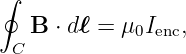
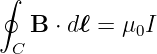
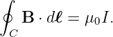
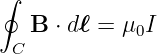
EM12 developed Ampère’s law for steady currents,

∮ B ⋅ dℓ = μ0Ienc, C

(1)

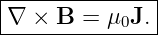
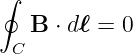
and its magnetostatic differential form,

∇ × B = μ0J.

(2)

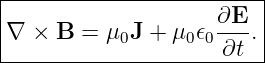
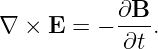
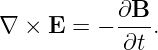
EM13 then introduced the first explicitly time-dependent Maxwell relation,

∂B ∇ × E = − ----. ∂t

(3)

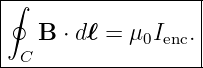
EM14 completes the second curl equation by asking a deceptively simple question:

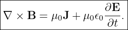
|-------------------------------------------------------------| What---happens-to-Amp--`ere’s-law-while-a-capacitor is-charging?-

(4)

The answer led Maxwell to introduce the displacement-current term. The result is the Ampère–Maxwell law, which makes Ampère’s circulation law consistent with charge conservation and provides the second dynamical field coupling required for electromagnetic waves [1, 2, 3, 4, 5].

1 The magnetostatic Ampère law

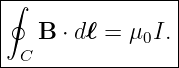
For steady currents,

|∮-----------------| | | | B ⋅ dℓ = μ0Ienc. --C-----------------

(5)

Using Stokes’ theorem,

∮ ∫ B ⋅ dℓ = (∇ × B ) ⋅ dA, C S

(6)

so the local magnetostatic law is

|--------------| -∇-×-B--=-μ0J.--

(7)

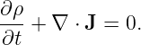
For steady current,

∂ρ ---= 0, ∂t

(8)

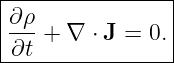
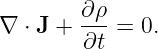
and the continuity equation reduces to

∇ ⋅ J = 0.

(9)

Thus a steady current has no local accumulation or depletion of charge.

2 The charging-capacitor problem

Consider a capacitor connected to a circuit while it is charging.

Conduction current flows through the wire toward one plate and away from the other. Choose a closed contour C that loops around the wire.

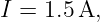
One surface S₁ bounded by C cuts through the wire. It encloses the conduction current I.

A second surface S₂, with the same boundary C, can be deformed so that it passes through the gap between the capacitor plates. No conduction current crosses the dielectric or vacuum gap.

If the original magnetostatic Ampère law were used without modification, the two surfaces would give

∮ B ⋅ dℓ = μ0I C

(10)

from S₁, but

∮ B ⋅ dℓ = 0 C

(11)

from S₂.

That cannot be correct because the line integral around the same contour C cannot have two different values.

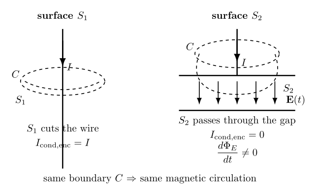
Figure. The charging-capacitor problem. Two surfaces share the same boundary C: one is pierced by conduction current, while the other passes through the capacitor gap. The original magnetostatic Ampère law cannot treat both surfaces consistently.

3 What changes in the capacitor gap?

Although conduction charge does not cross the gap, the electric field between the capacitor plates changes while the capacitor charges.

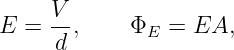
For an ideal parallel-plate capacitor, ignoring fringing,

E = σ-, 𝜖0

(12)

where σ = Q∕A is the plate charge density.

Therefore,

-Q-- E = 𝜖0A .

(13)

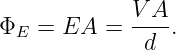
The electric flux through the plate area is

Φ_E	= EA	(14)
	= .	(15)

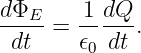
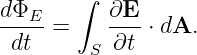
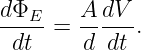
Differentiate with respect to time:

dΦE-- 1-dQ- dt = 𝜖0 dt .

(16)

Since

dQ I = ---, dt

(17)

we obtain

|------------| | dΦE-- | |𝜖0 dt = I. | -------------

(18)

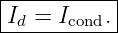
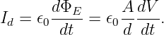
The changing electric flux through the capacitor gap has exactly the quantity needed to match the conduction current in the wire.

4 Maxwell’s displacement current

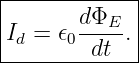
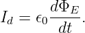
Maxwell defined the displacement current

|------------| |I = 𝜖 dΦE-.| --d---0--dt---

(19)

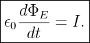
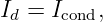
For an ideal charging capacitor,

|----------| |Id = Icond.| ------------

(20)

The terminology is historical. In a vacuum capacitor gap, displacement current does not mean that conduction charge physically crosses the gap. Instead, the quantity represents the magnetic-field source contribution associated with the changing electric flux.

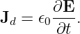
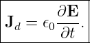
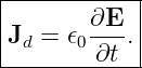
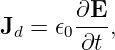
For a local electric field, the displacement-current density is

|------------| |J = 𝜖 ∂E- .| --d----0-∂t--|

(21)

Its SI units are

A/m2,

(22)

the same as an ordinary conduction current density.

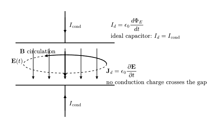
Figure. Between the capacitor plates, a changing electric field produces a displacement-current density J_d = 𝜖₀∂E∕∂t. It contributes to magnetic-field circulation even though no conduction charge crosses the gap.

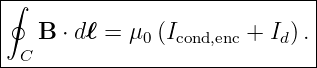
5 The Ampère–Maxwell integral law

The corrected circulation law is

|∮---------------------------------| | dΦE-- | | C B ⋅ d ℓ = μ0Icond,enc + μ0𝜖0 dt .| -----------------------------------

(23)

Equivalently,

|∮-----------------------------| | B ⋅ dℓ = μ0(Icond,enc + Id).| --C----------------------------|

(24)

Now return to the charging capacitor.

For a surface cutting the wire,

Icond,enc = I, Id = 0

(25)

for that simple surface choice.

For a surface passing through the capacitor gap,

Icond,enc = 0, Id = I.

(26)

Both surfaces therefore give the same magnetic circulation:

|∮---------------| | | | B ⋅ dℓ = μ0I.| --C---------------

(27)

The surface ambiguity is removed.

6 Example 1: displacement current in a charging capacitor

A capacitor has capacitance

C = 2.0μF

(28)

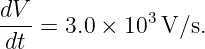
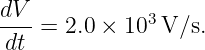
and its voltage increases at the rate

dV- 3 dt = 3.0 × 10 V/s.

(29)

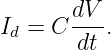
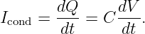
For a capacitor,

Q = CV,

(30)

I = dQ- = C dV-. cond dt dt

(31)

Thus,

I_cond	= (2.0 × 10⁻⁶)(3.0 × 10³)	(32)
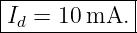
	= 6.0 × 10⁻³ A.	(33)

Therefore,

|--------------------| |Id = Icond = 6.0mA. | ----------------------

(34)

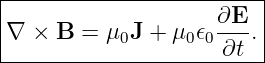
7 The differential Ampère–Maxwell equation

Apply Stokes’ theorem:

∮ ∫ B ⋅ dℓ = (∇ × B ) ⋅ dA. C S

(35)

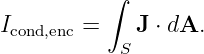
The enclosed conduction current is

∫ Icond,enc = J ⋅ dA. S

(36)

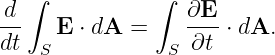
For a fixed surface,

∫ dΦE-- ∂E- dt = S ∂t ⋅ dA.

(37)

Therefore,

∫ ∫ ( ) ∂E- S(∇ × B ) ⋅ dA = S μ0J + μ0𝜖0 ∂t ⋅ dA.

(38)

For arbitrary fixed surfaces,

|------------------------| |∇ × B = μ0J + μ0 𝜖0∂E-.| ---------------------∂t---

(39)

This is the differential Ampère–Maxwell equation.

8 Why the Maxwell term is required by charge conservation

The divergence of any curl is zero:

∇ ⋅ (∇ × B ) = 0.

(40)

Take the divergence of the Ampère–Maxwell equation:

∂-- 0 = μ0∇ ⋅ J + μ0𝜖0∂t(∇ ⋅ E).

(41)

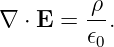
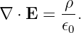
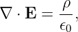
Gauss’s Law gives

∇ ⋅ E = ρ-. 𝜖0

(42)

Substitute:

0	= μ₀∇⋅ J + μ₀𝜖₀	(43)
	= μ₀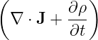.	(44)

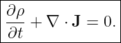
Therefore,

|----------------| |∂ρ- | |∂t + ∇ ⋅ J = 0.| -----------------

(45)

This is exactly the local charge-continuity equation introduced in EM08.

Thus the Maxwell correction is not an optional refinement. It is required for consistency with local charge conservation.

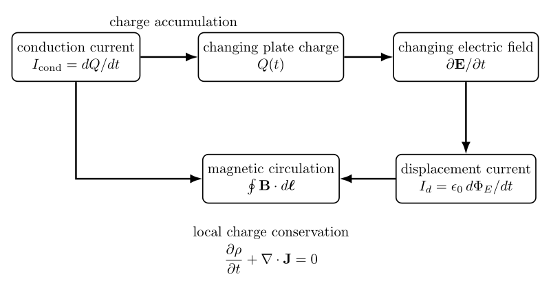
Figure. In a charging capacitor, conduction current in the wire and displacement current through the gap form a continuous source for magnetic-field circulation. The equality is another expression of charge conservation.

9 Magnetic field inside an ideal capacitor gap

Consider circular capacitor plates of radius R carrying charging current I. Assume the electric field in the gap is uniform over the plate area and neglect fringing.

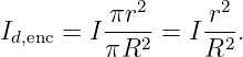
The total displacement current through the full plate area is

Id = I.

(46)

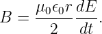
For a circular Amperian path of radius r < R centered on the capacitor axis, only the electric flux inside radius r is enclosed.

Because the displacement-current density is uniform,

πr2 r2 Id,enc = I---2 = I -2-. πR R

(47)

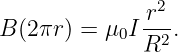
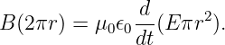
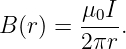
By symmetry, B is tangent to the circular path and has constant magnitude B(r). Ampère–Maxwell gives

2 B (2πr) = μ0I r--. R2

(48)

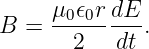
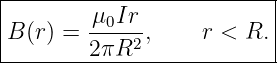
Therefore,

|--------------------------| | μ0Ir | |B (r) = ----2, r < R. | ---------2πR---------------

(49)

Inside the ideal gap, the magnetic field increases linearly with radius.

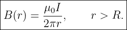
For r > R, the entire displacement current is enclosed:

|------------------------| | μ0I- | |B (r) = 2πr, r > R. | -------------------------

(50)

This is the same exterior radial dependence as for a long straight current.

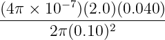
10 Example 2: field inside the capacitor gap

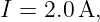
Let

I = 2.0A, R = 0.10 m, r = 0.040 m.

(51)

Since r < R,

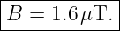
B	=	(52)
	=	(53)
	= 1.6 × 10⁻⁶ T.	(54)

Therefore,

|------------| -B-=--1.6-μT.-|

(55)

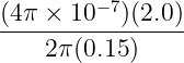
11 Example 3: field outside the plate radius

Using the same charging current,

I = 2.0A,

(56)

but at

r = 0.15m > R,

(57)

the full displacement current is enclosed:

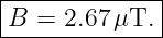
B	=	(58)
	=	(59)
	= 2.67 × 10⁻⁶ T.	(60)

Thus,

|-------------| B = 2.67μT. | ---------------

(61)

12 Displacement-current density in a time-varying electric field

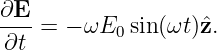
The local displacement-current density is

|------------| | ∂E | |Jd = 𝜖0-∂t .| -------------

(62)

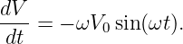
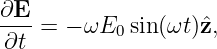
Suppose

E (t) = E0 cos(ωt)ˆz.

(63)

Then

∂E- ∂t = − ωE0 sin(ωt )ˆz,

(64)

|------------------------| Jd-(t)-=-−-𝜖0ωE0-sin(ωt)ˆz.-

(65)

Its peak magnitude is

|------------| Jd0-=-𝜖0ωE0.--

(66)

Thus higher-frequency electric-field variation produces a larger displacement-current density for the same field amplitude.

13 Example 4: sinusoidal displacement-current density

Let

E = 100 V/m, f = 1.0MHz. 0

(67)

Then

6 ω = 2πf = 6.283 × 10 rad/s.

(68)

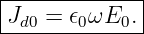
The peak displacement-current density is

J_d0	= 𝜖₀ωE₀	(69)
	= (8.854 × 10⁻¹²)(6.283 × 10⁶)(100)	(70)
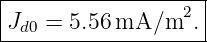
	= 5.56 × 10⁻³ A/m².	(71)

Therefore,

|------------------| | 2 | Jd0-=-5.56-mA/m---.-

(72)

14 Example 5: continuity-equation check

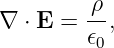
Start from

∇ × B = μ J + μ 𝜖 ∂E-. 0 0 0∂t

(73)

Take the divergence:

∂ 0 = μ0∇ ⋅ J + μ0𝜖0--(∇ ⋅ E). ∂t

(74)

Using Gauss’s law,

ρ- ∇ ⋅ E = 𝜖0 ,

(75)

gives

∂ρ ∇ ⋅ J + ---= 0. ∂t

(76)

Thus the Ampère–Maxwell equation automatically contains the local continuity equation once Gauss’s law is included.

15 The current-free vacuum case

In a region containing no conduction current,

J = 0.

(77)

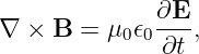
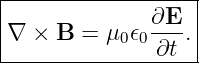
The Ampère–Maxwell equation becomes

|------------------| | ∂E | |∇ × B = μ0 𝜖0 ---.| ---------------∂t--

(78)

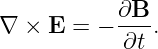
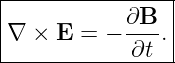
EM13 gave the complementary dynamical curl law:

|-----------∂B---| |∇ × E = − ----.| -------------∂t--|

(79)

The two time-dependent curl equations now form a coupled pair:

|------------------------------------| |∂B ∂E | |∂t--−→ ∇ × E, -∂t − → ∇ × B. | --------------------------------------

(80)

This reciprocal coupling is the essential local mechanism behind self-propagating electromagnetic waves.

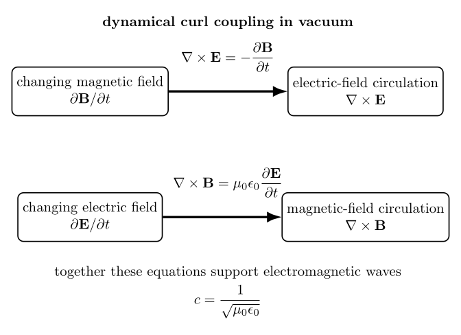
Figure. The two dynamical curl laws. A changing magnetic field is tied to electric-field circulation, while a changing electric field is tied to magnetic-field circulation.

16 Example 6: magnetic circulation from a changing electric field

Suppose a spatially uniform electric field fills a circular region and changes at the rate

dE 11 -dt = 5.0 × 10 V/ (m s).

(81)

Choose a circular contour of radius

− 2 r = 2.0 × 10 m

(82)

inside that region.

Ampère–Maxwell gives

d B(2πr ) = μ0𝜖0--(E πr2). dt

(83)

Therefore,

B = μ0-𝜖0rdE-. 2 dt

(84)

Using

− 17 2 2 μ0𝜖0 ≈ 1.113 × 10 s ∕m ,

(85)

we obtain

B	= (5.0 × 10¹¹)	(86)
	= 5.56 × 10⁻⁸ T.	(87)

Thus,

|------------------| B = 5.56 × 10−8 T.| --------------------

(88)

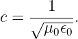
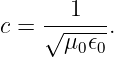
17 The electromagnetic speed scale

The combination

μ0𝜖0

(89)

appears in the Ampère–Maxwell equation.

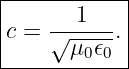
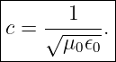
It defines a speed scale

|-------1----| |c = √-----. | -------μ0𝜖0--|

(90)

Using the vacuum constants,

|--------------------| |c ≈ 2.998 × 108m/s. | ----------------------

(91)

This is the speed of light in vacuum.

The appearance of the speed of light from purely electromagnetic constants was one of Maxwell’s central results. The next stages of this series will show explicitly how the coupled curl equations produce wave equations whose propagation speed is exactly this value.

18 Example 7: computing the electromagnetic speed

Using

−6 μ0 ≈ 1.25663706 × 10 H/m

(92)

and

𝜖 ≈ 8.85418781 × 10 −12F/m, 0

(93)

we find

c	=	(94)
	≈ 2.998 × 10⁸ m/s.	(95)

Thus,

|--------------------| |c ≈ 299 792458 m/s. | ----------------------

(96)

19 Common mistakes

Mistake: interpreting displacement current as ordinary charge crossing a vacuum capacitor gap. No conduction charge crosses the ideal gap.
Mistake: using the magnetostatic Ampère law unchanged when electric flux varies with time.
Mistake: forgetting that different surfaces spanning the same contour must give the same magnetic circulation.
Mistake: confusing electric flux Φ_E with electric field magnitude E.
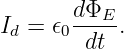
Mistake: forgetting the factor 𝜖₀ in I_d = 𝜖₀ dΦ_E∕dt.
Mistake: assuming displacement current exists only inside capacitors. The local term 𝜖₀∂E∕∂t exists wherever the electric field varies in time.
Mistake: dropping the conduction-current term in material regions where J≠0.
Mistake: treating μ₀𝜖₀ as an arbitrary constant product rather than the quantity that sets the vacuum electromagnetic propagation speed.

Part I: Exercises

All exercises are stated here before any worked solution. Attempt the complete set before proceeding to Part II.

Exercise 1: displacement current from changing electric flux

The electric flux through a surface changes at the rate

dΦE--= 8.0 × 108 V m/s. dt

(97)

Find the displacement current

I = 𝜖 dΦE-. d 0 dt

(98)

Exercise 2: charging capacitor from capacitance and voltage rate

A capacitor has

C = 5.0μF

(99)

and its voltage rises at

dV- = 2.0 × 103V/s. dt

(100)

Find:

the conduction current in the wires;
the displacement current through the capacitor gap.

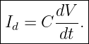
Exercise 3: derive displacement current for a parallel-plate capacitor

A vacuum parallel-plate capacitor has plate area A, separation d, and voltage V (t).

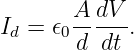
Using

E = V-, Φ = EA, d E

(101)

derive

A dV Id = 𝜖0-----. d dt

(102)

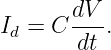
Then identify the capacitance C and show that

dV Id = C ---. dt

(103)

Exercise 4: magnetic field inside a charging capacitor gap

Circular capacitor plates have radius

R = 0.080m.

(104)

The charging current is

I = 1.5A.

(105)

Neglect fringing. Find the magnetic-field magnitude in the gap at radius

r = 0.030 m, r < R.

(106)

Exercise 5: magnetic field outside the plate radius

Using the same charging current

I = 1.5A,

(107)

find the magnetic-field magnitude at

r = 0.12 m, r > R.

(108)

Exercise 6: sinusoidal displacement-current density

A uniform electric field is

E (t) = (250 V/m )cos(2πf t)ˆz,

(109)

with

f = 2.0 MHz.

(110)

Find:

J_d(t);
the peak displacement-current density.

Exercise 7: displacement-current direction and magnetic circulation

At a particular instant,

∂E 10 --- = + (4.0 × 10 V/ (m s))ˆz. ∂t

(111)

Determine:

the direction of J_d;
whether the associated magnetic-field circulation is clockwise or counterclockwise when viewed from the +z side.

Exercise 8: surface independence around a charging capacitor

A contour C surrounds a wire carrying charging current I into a capacitor.

Surface S₁ cuts the wire. Surface S₂ bulges between the capacitor plates.

State the values of

Icond,enc

(112)

and

Id

(113)

for each surface, and show that both surfaces give the same Ampère–Maxwell circulation.

Exercise 9: derive the differential Ampère–Maxwell law

Starting from

∮ ∫ ∫ d- B ⋅ dℓ = μ0 J ⋅ dA + μ0 𝜖0 dt E ⋅ dA, C S S

(114)

for a fixed surface, use Stokes’ theorem to derive

∇ × B = μ J + μ 𝜖 ∂E-. 0 0 0∂t

(115)

Exercise 10: derive charge continuity

Starting from the differential Ampère–Maxwell equation, take the divergence and use Gauss’s law,

∇ ⋅ E = ρ-, 𝜖0

(116)

to derive

∂ρ ---+ ∇ ⋅ J = 0. ∂t

(117)

Exercise 11: magnetic field from a changing electric field in vacuum

A spatially uniform electric field fills a circular region and changes at the rate

dE 12 --- = 3.0 × 10 V/ (m s). dt

(118)

Find the magnetic-field magnitude on a circular contour of radius

r = 1.0 × 10− 2m

(119)

lying entirely inside the changing-field region.

Exercise 12: conduction current versus displacement current

For an ideal vacuum capacitor that is charging, explain precisely why

Id = Icond

(120)

does not mean that ordinary conduction charge crosses the vacuum gap.

Your answer should distinguish charge transport from the field term 𝜖₀∂E∕∂t.

Exercise 13: sinusoidally driven capacitor

A capacitor with capacitance

C = 100 pF

(121)

has applied voltage

V (t) = V0 cos(ωt),

(122)

where

V0 = 5.0V, f = 10MHz, ω = 2πf.

(123)

Find:

the displacement current I_d(t);
its peak magnitude.

Exercise 14: the electromagnetic speed scale

Using

μ0 = 1.25663706 × 10 −6H/m

(124)

and

𝜖0 = 8.85418781 × 10 −12F/m,

(125)

compute

c = √--1--. μ0𝜖0

(126)

Then explain why the appearance of this speed in the coupled Maxwell curl equations is the key bridge from circuit-like Electromagnetism to electromagnetic waves.

Part II: Complete Worked Solutions

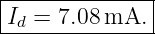
Solution 1: displacement current from changing electric flux

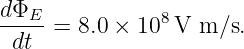
Use

I = 𝜖 dΦE-. d 0 dt

(127)

Therefore,

I_d	= (8.854 × 10⁻¹²)(8.0 × 10⁸)	(128)
	= 7.08 × 10⁻³ A.	(129)

Thus,

|--------------| -Id =-7.08mA.--|

(130)

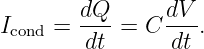
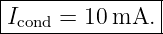
Solution 2: charging capacitor from capacitance and voltage rate

For a capacitor,

Q = CV.

(131)

Differentiate:

I = dQ- = C dV-. cond dt dt

(132)

Thus,

I_cond	= (5.0 × 10⁻⁶)(2.0 × 10³)	(133)
	= 1.0 × 10⁻² A.	(134)

So,

|--------------| -Icond-=-10-mA.--

(135)

For an ideal charging capacitor,

Id = Icond,

(136)

therefore,

|------------| -Id =-10mA.---

(137)

Solution 3: derive displacement current for a parallel-plate capacitor

The field is

V E = --. d

(138)

The electric flux is

V-A- ΦE = EA = d .

(139)

Differentiate:

dΦE A dV -----= -----. dt d dt

(140)

Therefore,

Id = 𝜖0d-ΦE-= 𝜖0A-dV-. dt d dt

(141)

For a vacuum parallel-plate capacitor,

C = 𝜖0A-. d

(142)

Hence,

|-----------| | dV | Id = C ---. | --------dt---

(143)

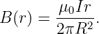
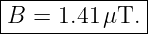
Solution 4: magnetic field inside a charging capacitor gap

For r < R,

μ0Ir-- B (r) = 2πR2 .

(144)

Substitute:

B	=	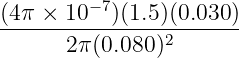(145)
	= 1.41 × 10⁻⁶ T.	(146)

Therefore,

|-------------| B = 1.41μT. | ---------------

(147)

Solution 5: magnetic field outside the plate radius

For r > R, the full displacement current is enclosed:

B (r) = μ0I-. 2πr

(148)

Thus,

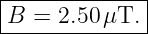
B	=	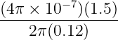(149)
	= 2.50 × 10⁻⁶ T.	(150)

Therefore,

|-------------| B--=-2.50μT.---

(151)

Solution 6: sinusoidal displacement-current density

The field is

E (t) = E0 cos(ωt)ˆz,

(152)

with

E0 = 250 V/m, ω = 2π(2.0 × 106).

(153)

Differentiate:

∂E --- = − ωE0 sin(ωt )ˆz. ∂t

(154)

Therefore,

|------------------------| Jd-(t)-=-−-𝜖0ωE0-sin(ωt)ˆz.-

(155)

The peak magnitude is

J_d0	= 𝜖₀ωE₀	(156)
	= (8.854 × 10⁻¹²)[2π(2.0 × 10⁶)](250)	(157)
	= 2.78 × 10⁻² A/m².	(158)

Hence,

|---------------−2-----2-| -Jd0 =-2.78-×--10--A/m---.-

(159)

Solution 7: displacement-current direction and magnetic circulation

Because

∂E Jd = 𝜖0--- , ∂t

(160)

and 𝜖₀ > 0, the displacement-current density points in the same direction as ∂E∕∂t.

Therefore,

|--------------------| |Jd points along + ˆz.| ----------------------

(161)

Using the right-hand rule, a current-like source in the +z direction produces counterclockwise magnetic circulation when viewed from the +z side.

Thus,

|--------------------------------------------------| -B-circulates counterclockwise-as-viewed-from--+--z.|

(162)

Solution 8: surface independence around a charging capacitor

For surface S₁ cutting the wire,

Icond,enc = I, Id = 0.

(163)

Hence,

∮ C B ⋅ dℓ = μ0I.

(164)

For surface S₂ passing through the capacitor gap,

Icond,enc = 0, Id = I

(165)

for the ideal charging capacitor.

Therefore,

∮ B ⋅ dℓ = μ0I C

(166)

again.

So,

|------------------∮---------------| | | both surfaces give B ⋅ dℓ = μ0I.| --------------------C---------------

(167)

Solution 9: derive the differential Ampère–Maxwell law

Start from

∮ ∫ ∫ d- C B ⋅ dℓ = μ0 S J ⋅ dA + μ0 𝜖0 dt S E ⋅ dA.

(168)

By Stokes’ theorem,

∮ ∫ B ⋅ dℓ = (∇ × B ) ⋅ dA. C S

(169)

For a fixed surface,

∫ ∫ d ∂E dt E ⋅ dA = -∂t ⋅ dA. S S

(170)

Therefore,

∫ [ ] ∇ × B − μ0J − μ0 𝜖0∂E- ⋅ dA = 0. S ∂t

(171)

Because the fixed surface is arbitrary,

|------------------------| |∇ × B = μ0J + μ0 𝜖0∂E-.| ---------------------∂t---

(172)

Solution 10: derive charge continuity

Start from

∇ × B = μ J + μ 𝜖 ∂E-. 0 0 0∂t

(173)

Take the divergence:

∂ ∇ ⋅ (∇ × B ) = μ0∇ ⋅ J + μ0𝜖0∂t(∇ ⋅ E ).

(174)

The divergence of a curl is zero:

∂ 0 = μ0∇ ⋅ J + μ0𝜖0--(∇ ⋅ E). ∂t

(175)

Use Gauss’s law,

ρ- ∇ ⋅ E = 𝜖 . 0

(176)

Then

0	= μ₀∇⋅ J + μ₀𝜖₀	(177)
	= μ₀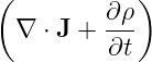.	(178)

Therefore,

|----------------| |∂ρ | |---+ ∇ ⋅ J = 0.| -∂t--------------

(179)

Solution 11: magnetic field from a changing electric field in vacuum

For a circular contour lying inside a region of uniform changing electric field,

B(2πr ) = μ 𝜖 d-(E πr2). 0 0dt

(180)

Thus,

μ0 𝜖0rdE B = --2----dt .

(181)

Substitute

− 17 2 2 μ0𝜖0 ≈ 1.113 × 10 s ∕m ,

(182)

B	= (3.0 × 10¹²)	(183)
	= 1.67 × 10⁻⁷ T.	(184)

Therefore,

|-------------−7---| B--=-1.67-×-10---T.-

(185)

Solution 12: conduction current versus displacement current

The equality

Id = Icond

(186)

for an ideal charging capacitor is a statement about the source term in Ampère–Maxwell circulation, not about identical microscopic transport mechanisms.

In the wire, ordinary mobile charge crosses a material cross section. This is conduction current.

In the ideal vacuum gap, those conduction charges do not cross from one plate to the other. Instead, the plate charge changes, causing the electric field in the gap to change. The associated field term is

J = 𝜖 ∂E- . d 0 ∂t

(187)

Its surface integral equals the conduction current for the ideal capacitor:

|----------------------------------------------------------| -Id =-Icond,--but--the-microscopic-mechanisms---are-different.-|

(188)

Solution 13: sinusoidally driven capacitor

The voltage is

V (t) = V0 cos(ωt).

(189)

For a capacitor,

Id = C dV-. dt

(190)

Differentiate:

dV- = − ωV sin(ωt). dt 0

(191)

Therefore,

|----------------------| Id(t) =-−-ωCV0-sin(ωt).-

(192)

The peak magnitude is

I = ωCV . d0 0

(193)

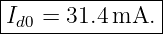
Using

7 7 ω = 2π (10 ) = 6.283 × 10 rad/s,

(194)

I_d0	= (6.283 × 10⁷)(100 × 10⁻¹²)(5.0)	(195)
	= 3.14 × 10⁻² A.	(196)

Thus,

|--------------| Id0-=-31.4-mA.--

(197)

Solution 14: the electromagnetic speed scale

Compute

c = ---1--. √ μ0𝜖0-

(198)

Using the given values,

c	=	(199)
	≈ 2.998 × 10⁸ m/s.	(200)

Therefore,

|--------------------| |c ≈ 2.998 × 108m/s. | ----------------------

(201)

In a current-free region,

∂E ∇ × B = μ0 𝜖0 ---, ∂t

(202)

while Faraday’s law gives

∇ × E = − ∂B--. ∂t

(203)

Each changing field is therefore tied to spatial circulation of the other. When these coupled equations are combined with the vector-calculus identities developed earlier in the series, they generate wave equations with propagation speed

|-------1----| |c = √-----. | -------μ0𝜖0--|

(204)

This is the direct bridge from Maxwell’s field equations to electromagnetic waves.

20 What EM14 adds to the series

EM13 established

∇ × E = − ∂B--. ∂t

(205)

EM14 completes the dynamical partner,

|------------------------| | ∂E | |∇ × B = μ0J + μ0 𝜖0---.| ---------------------∂t---

(206)

In vacuum, where J = 0, the two curl equations become mutually coupled time-dependent field equations.

The next natural step is to gather the four Maxwell equations together and then derive the electromagnetic wave equation directly from them.

References

[1] David J. Griffiths, Introduction to Electrodynamics, 4th ed., Cambridge University Press, 2017.

[2] Edward M. Purcell and David J. Morin, Electricity and Magnetism, 3rd ed., Cambridge University Press, 2013.

[3] Samuel J. Ling, Jeff Sanny, and William Moebs, University Physics, Volume 2, OpenStax, 2016, sections on Maxwell’s equations, displacement current, and electromagnetic waves.

[4] Richard P. Feynman, Robert B. Leighton, and Matthew Sands, The Feynman Lectures on Physics, Volume II, Addison-Wesley, 1964, chapters on Maxwell’s equations, displacement current, and electromagnetic radiation.

[5] Massachusetts Institute of Technology, 8.02 Physics II: Electricity and Magnetism, MIT OpenCourseWare, materials on Ampère–Maxwell law, displacement current, capacitors, and Maxwell’s equations.

"Electromagnetic Waves: Ampere-Maxwell Law and Displacement Current" is owned by bloftin.
(view preamble)