Celestial Mechanics: Newtonian Gravitation - Worked Problems and Complete Solutions
CM01 introduced Newton’s universal law of gravitation as the dynamical starting point for
celestial mechanics. This companion article develops fluency with that law before gravitational
potential, orbital energy, or conic-section dynamics are introduced.
The problems begin with direct force-law and field-strength calculations and then progress to
vector components, inverse-square scaling, two-body acceleration, superposition, balance points,
continuous spherical mass distributions, and a numerical implementation of the Newtonian
field.
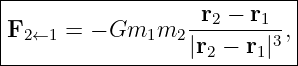
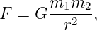
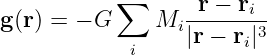
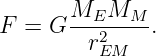
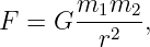
The central equations are
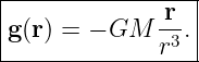
and, for The Gravitational Field produced by a point source mass M,
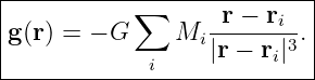
For several sources,
Unless otherwise stated, use
and
Part I: Exercises
Exercise 1: Earth–Moon gravitational force
Treat Earth and the Moon as point masses separated by their mean center-to-center
distance.
- Compute the magnitude of the gravitational force Earth exerts on the Moon.
- State the magnitude of the force the Moon exerts on Earth.
- Explain why the two bodies do not have equal accelerations even though the force
magnitudes are equal.
Exercise 2: gravitational field strength at Earth’s surface and at 400 km altitude
Using the point-mass/spherical-Earth approximation, calculate
- the gravitational field magnitude at Earth’s mean surface;
- the gravitational field magnitude at altitude h = 400 km;
- the ratio g(RE + h)∕g(RE).
Explain why astronauts in low Earth orbit are not beyond Earth’s gravity.
Exercise 3: inverse-square scaling without repeating the full calculation
At distance r from a point mass, the gravitational field magnitude is g.
Determine the field magnitude if
- the distance is doubled;
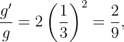
- the distance is tripled;
- the source mass is doubled while the distance is tripled;
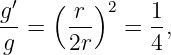
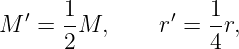
- the source mass is reduced to one half while the distance is reduced to one quarter.
Do this using ratios rather than substituting G numerically.
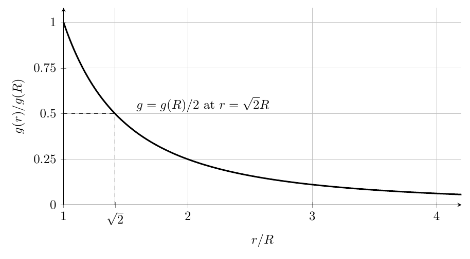
Figure. The normalized point-mass field follows g(r)∕g(R) = (R∕r)2. At r =  R, the
field has fallen to one half its value at R.
R, the
field has fallen to one half its value at R.
Exercise 4: force versus field and cancellation of test mass
At altitude 1000 km above Earth’s mean radius:
- calculate the gravitational field magnitude;
- calculate the force on a 1.00 kg test mass;
- calculate the force on a 1000 kg spacecraft;
- calculate the acceleration of each object.
Use the result to explain the difference between gravitational force and gravitational
field.
Exercise 5: vector gravitational force from Cartesian coordinates
Two point masses have
Their positions are
and
Find
- the relative-position vector r = r2 − r1;
- its magnitude and unit vector;
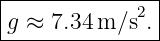
- the gravitational force vector on m2 due to m1;
- the force vector on m1 due to m2.
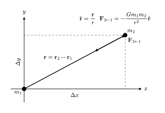
Figure. Once the relative-position vector is defined, the minus sign in the Newtonian
vector force law makes the force on body 2 point back toward body 1.
Exercise 6: equal force, unequal acceleration in the Earth–Moon system
Using the force from Exercise 1:
- calculate Earth’s acceleration toward the Moon;
- calculate the Moon’s acceleration toward Earth;
- calculate the ratio aM∕aE;
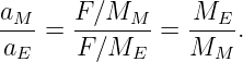
- show that this ratio is equal to ME∕MM.
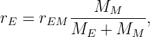
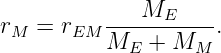
Then calculate the distances of Earth and Moon from their common center of mass
using
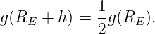
Exercise 7: altitude where Earth’s gravitational field is one half of its surface value
Find the altitude h above Earth’s mean surface where
Do not substitute numerical constants until after solving symbolically for h.
Exercise 8: recover the gravitational parameter and source mass from a field measurement
At distance
from the center of an approximately spherical body, a gravitational field magnitude
is measured.
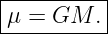
- Determine the body’s gravitational parameter μ = GM.
- Determine the body’s mass M.
- Explain why orbital mechanics often works directly with μ rather than with G and M
separately.
Exercise 9: the Sun’s field at Earth and the force on Earth
At one astronomical unit:
- calculate the magnitude of the Sun’s gravitational field;
- calculate the gravitational force magnitude on Earth;
- compare the solar field at Earth with Earth’s field at its own surface by computing the
ratio g⊙(1 AU)∕gE(RE).
Explain why a comparatively small acceleration can control an orbit over astronomical time
scales.
Exercise 10: superposition above two equal masses
Two equal masses
are located at
with
An observation point is at
- Find the field vector from each source at P.
- Show explicitly that the horizontal components cancel.
- Find the net gravitational field vector and magnitude.
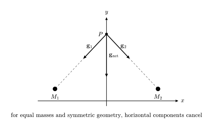
Figure. Symmetry can simplify superposition. For equal masses placed symmetrically
about the vertical axis, horizontal field components cancel at points on that axis.
Exercise 11: zero-field point between two unequal masses
Two masses M1 and M2 are separated by distance d, with M1 > M2. Consider only their
Newtonian gravitational fields along the line joining them.
- Derive the position x, measured from M1, where the net gravitational field is zero
between the masses.
- Apply the result to the Earth–Moon pair.
- Give the distance of this zero-field point from the Moon’s center.
- Explain why this point is not the Earth–Moon L1 Lagrange point.
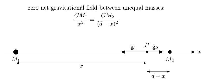
Figure. Between two unequal masses, the zero-field point lies closer to the smaller source.
This is a gravitational-field balance only; a rotating-frame equilibrium requires additional
inertial terms.
Exercise 12: surface gravity of a uniform-density spherical body
A spherical body has uniform density ρ and radius R.
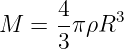
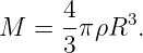
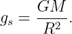
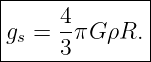
- Use
to derive a formula for its surface gravitational field gs in terms of ρ and R.
- Evaluate the result for
Exercise 13: dimensional analysis of G and μ
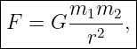
Starting from
derive the SI dimensions of G.
Then define
and determine the dimensions of μ.
Finally show that
has dimensions of acceleration.
Exercise 14: Julia implementation of Newtonian gravitational superposition
Write a Julia function that evaluates
for an arbitrary list of point masses.
Use the two equal masses from Exercise 10 and verify numerically that
- the field at the midpoint (0, 0) is zero;
- the field at (0, 106 m) has zero x component;
- its y component agrees with Exercise 10.
Part II: Complete Worked Solutions
Solution 1: Earth–Moon gravitational force
Newton’s scalar force law gives
Substitute the numerical values:
| F | = (6.67430 × 10⁻¹¹) | (28)
|
| ≈ 1.98 × 10²⁰ N. | (29) |
Therefore
Newton’s third law requires an equal and opposite force on Earth:
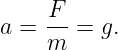
The accelerations differ because
The same force divided by the much smaller lunar mass produces a much larger acceleration of the
Moon than of Earth.
Solution 2: gravitational field strength at Earth’s surface and at 400 km altitude
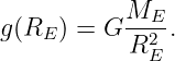
At Earth’s surface,
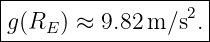
Thus
| g(RE) | = (6.67430 × 10⁻¹¹)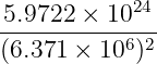 | (34)
|
| ≈ 9.8203 m/s2. | (35) |
Hence
At altitude h = 400 km,
Therefore
| g(RE + h) | = G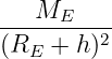 | (38)
|
| ≈ 8.6943 m/s2. | (39) |
Thus
The ratio is
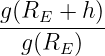 | = 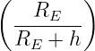 2 2 | (41)
|
| ≈ 0.885. | (42) |
So
Gravity at this altitude is still almost 89% of its surface value. Orbiting astronauts appear
weightless because they and their spacecraft are in continuous free fall, not because gravity has
become negligible.
Solution 3: inverse-square scaling without repeating the full calculation
Because
ratios can be formed directly.
If r′ = 2r,
so
If r′ = 3r,
If M′ = 2M and r′ = 3r,
so
Finally, if
then
 | =   2 2 | (51)
|
| =  (16) (16) | (52)
|
| = 8. | (53) |
Therefore
The inverse-square dependence can overwhelm a moderate change in source mass because distance
enters quadratically.
Solution 4: force versus field and cancellation of test mass
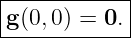
At altitude 1000 km,
The gravitational field is
| g | = G | (56)
|
| ≈ 7.3365 m/s2. | (57) |
Thus
For a 1.00 kg mass,
so
For a 1000 kg spacecraft,
so
The acceleration of either body is
Therefore
The force scales with test mass; the gravitational field does not. Dividing the force by inertial mass
removes the test mass from the acceleration.
Solution 5: vector gravitational force from Cartesian coordinates
The relative vector is
| r | = r2 − r1 | (65)
|
| = (3.00 × 10⁶x + 4.00 × 10⁶y) m. | (66) |
Its magnitude is
| r | =  | (67)
|
| = 5.00 × 10⁶ m. | (68) |
Hence
The force magnitude is
| F | = G | (70)
|
| = (6.67430 × 10⁻¹¹)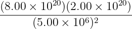 | (71)
|
| = 4.27155 × 10¹⁷ N. | (72) |
The force on body 2 points opposite r:
| F2←1 | = −Fr | (73)
|
| = −(4.27155 × 10¹⁷)(0.600x + 0.800y). | (74) |
Therefore
Newton’s third law gives
Solution 6: equal force, unequal acceleration in the Earth–Moon system
Using
Earth’s acceleration is
| aE | =  | (78)
|
| ≈ 3.3163 × 10⁻⁵ m/s2. | (79) |
Thus
The Moon’s acceleration is
| aM | =  | (81)
|
| ≈ 2.6976 × 10⁻³ m/s2. | (82) |
Thus
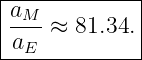
The acceleration ratio is
Numerically,
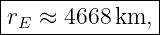
Now compute the center-of-mass distances:
| rE | = rEM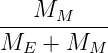 | (86)
|
| ≈ 4.668 × 10⁶ m, | (87) |
and
| rM | = rEM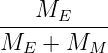 | (88)
|
| ≈ 3.7973 × 10⁸ m. | (89) |
Therefore
Both bodies move about their common center of mass; the center lies much closer to Earth because
Earth is much more massive.
Solution 7: altitude where Earth’s gravitational field is one half of its surface value
Write
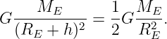
Cancel GME:
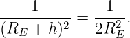
Invert both sides:
Take the positive square root:
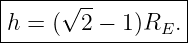
Therefore
Numerically,
| h | = ( − 1)(6.371 × 10⁶) − 1)(6.371 × 10⁶) | (97)
|
| ≈ 2.639 × 10⁶ m. | (98) |
Thus
The gravitational field does not fall to one half until the radial distance has increased to  times
Earth’s radius.
times
Earth’s radius.
Solution 8: recover the gravitational parameter and source mass from a field measurement
For a spherical source,
Therefore
Substitute the measurement:
| μ | = (8.13475)(7.00 × 10⁶)2 | (102)
|
| ≈ 3.98603 × 10¹⁴ m3∕s2. | (103) |
Thus
The mass is
Hence
| M | = 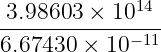 | (106)
|
| ≈ 5.9722 × 1024 kg. | (107) |
Therefore
This is essentially Earth’s mass. Orbital dynamics often uses μ directly because the equations of
motion depend on the product GM, and μ can be determined very accurately from orbital
observations even when G and M separately are less precisely known.
Solution 9: the Sun’s field at Earth and the force on Earth
The solar field at one astronomical unit is
| g⊙ | = G | (109)
|
| = (6.67430 × 10⁻¹¹)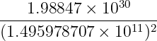 | (110)
|
| ≈ 5.9303 × 10⁻³ m/s2. | (111) |
Thus
The force on Earth is
| F | = MEg⊙ | (113)
|
| ≈ (5.9722 × 1024)(5.9303 × 10⁻³) | (114)
|
| ≈ 3.542 × 10²² N. | (115) |
Therefore
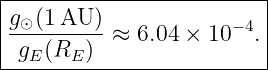
The ratio to Earth’s surface field is
 | = 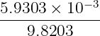 | (117)
|
| ≈ 6.04 × 10⁻⁴. | (118) |
So
The solar acceleration is small compared with surface gravity, but it acts continuously. Celestial
motion is controlled by sustained acceleration over long times rather than by requiring a large
instantaneous acceleration.
Solution 10: superposition above two equal masses
The two source positions are
and the observation point is
For the left source,
For the right source,
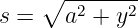
Each source is a distance
from P.
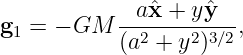
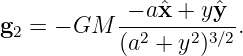
The two field contributions are
and
For the numerical values in the problem, each Cartesian component has magnitude
Thus
and
Add them:
| gnet | = g1 + g2 | (130)
|
| = −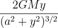 y. y. | (131) |
The x components cancel exactly.
For
we obtain
| |gnet| | =  | (133)
|
| ≈ 4.7194 × 10⁻³ m/s2. | (134) |
Therefore
Symmetry removes one component before any difficult arithmetic is required.
Solution 11: zero-field point between two unequal masses
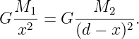
Let the balance point lie a distance x from M1. Its distance from M2 is d − x.
Between the masses the two gravitational fields point in opposite directions. Zero net field requires
equal magnitudes:
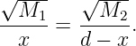
Cancel G and take the positive square root:
Cross multiply:
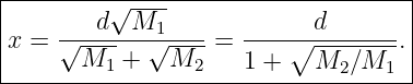
Thus
so
For Earth and Moon,
| x | = 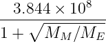 | (141)
|
| ≈ 3.4603 × 10⁸ m. | (142) |
Therefore the zero-field point is
Its distance from the Moon is
| rM,P | = rEM − x | (144)
|
| ≈ 3.8367 × 10⁷ m, | (145) |
or
This point is not L1. The L1 point is an equilibrium in a frame rotating with the Earth–Moon
system and therefore includes the rotating-frame inertial terms associated with the required orbital
angular speed. Exercise 11 balances only the two Newtonian gravitational fields in an inertial
description.
Solution 12: surface gravity of a uniform-density spherical body
For a uniform sphere,
The surface field is
Substitute the mass:
Therefore
For
we obtain
| gs | =  π(6.67430 × 10⁻¹¹)(5514)(106) π(6.67430 × 10⁻¹¹)(5514)(106) | (153)
|
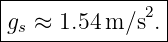
| ≈ 1.5416 m/s2. | (154) |
Thus
At fixed density, surface gravity scales linearly with radius because total mass grows as R3 while
the inverse-square field divides by R2.
Solution 13: dimensional analysis of G and μ
From
solve dimensionally for G:
Since
we obtain
| [G] | = 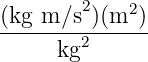 | (159)
|
| = m3kg−1s−2. | (160) |
Therefore
For
we have
Thus
Finally,
which is exactly the dimension of acceleration.
Solution 14: Julia implementation of Newtonian gravitational superposition
One direct implementation using three-component vectors is
using LinearAlgebra
using Printf

const G = 6.67430e-11

function gravity_field(r, masses, positions)
g = zeros(3)
for i in eachindex(masses)
dr = r - positions[i]
d = \href{https://physicslibrary.org/encyclopedia/NormInducedByInnerProduct.html}{norm(}dr)
g .+= -G * masses[i] * dr / d^3
end
return g
end

M = 1.0e20
masses = [M, M]
positions = [
[-1.0e6, 0.0, 0.0],
[ 1.0e6, 0.0, 0.0]
]

r_mid = [0.0, 0.0, 0.0]
r_top = [0.0, 1.0e6, 0.0]

g_mid = gravity_field(r_mid, masses, positions)
g_top = gravity_field(r_top, masses, positions)

println("g(midpoint) = ", g_mid)
println("g(top) = ", g_top)
@printf("|g(top)| = %.8e m/s^2\n", norm(g_top))
At the midpoint, symmetry gives
At the point directly above the midpoint, the two x components cancel numerically. The result
should be approximately
This agrees with the analytic superposition calculation in Exercise 10.
The implementation also exposes the mathematical structure that will later become
the Newtonian N-body problem: every source contributes a vector term proportional
to
1 What CM01E1 adds to the series
CM01 introduced the law. CM01E1 develops the ability to use it in several complementary
forms:
The exercises also establish several scaling ideas that recur throughout celestial mechanics:
and
The next main theory article, CM02, develops gravitational potential and potential energy. That
change of viewpoint converts the inverse-square vector field into a scalar potential and prepares the
later derivation of orbital-energy conservation.
References
[1] Bradley W. Carroll and Dale A. Ostlie, An Introduction to Modern Astrophysics, 2nd
ed., Pearson/Addison-Wesley, 2007.
[2] Herbert Goldstein, Charles Poole, and John Safko, Classical Mechanics, 3rd ed.,
Addison-Wesley, 2001.
[3] J. M. A. Danby, Fundamentals of Celestial Mechanics, 2nd ed., Willmann-Bell, 1988.
[4] Roger R. Bate, Donald D. Mueller, and Jerry E. White, Fundamentals of
Astrodynamics, Dover Publications, 1971.
[5] Isaac Newton, The Principia: Mathematical Principles of Natural Philosophy, trans.
I. Bernard Cohen and Anne Whitman, University of California Press, 1999.

![[parent]](https://images.physicslibrary.org/images/uparrow.png)


































































![[F-][r]2
[G] = [m ]2 .](https://images.physicslibrary.org/cache/objects/1250/make4ht/CelestialMechanicsNewtonianGravitationWorkedProblemsAndCompleteSolutions132x.png)
![2
[F ] = kg m/s ,](https://images.physicslibrary.org/cache/objects/1250/make4ht/CelestialMechanicsNewtonianGravitationWorkedProblemsAndCompleteSolutions133x.png)
![|-------3--−1-−-2-|
[G-] =-m-kg--s--.--](https://images.physicslibrary.org/cache/objects/1250/make4ht/CelestialMechanicsNewtonianGravitationWorkedProblemsAndCompleteSolutions135x.png)

![[μ] = (m3kg −1s−2)(kg) = m3s− 2.](https://images.physicslibrary.org/cache/objects/1250/make4ht/CelestialMechanicsNewtonianGravitationWorkedProblemsAndCompleteSolutions137x.png)
![|------------|
|[μ ] = m3 ∕s2.
--------------](https://images.physicslibrary.org/cache/objects/1250/make4ht/CelestialMechanicsNewtonianGravitationWorkedProblemsAndCompleteSolutions138x.png)
![[ μ ] m3 ∕s2 2
-2 = ----2- = m/s ,
r m](https://images.physicslibrary.org/cache/objects/1250/make4ht/CelestialMechanicsNewtonianGravitationWorkedProblemsAndCompleteSolutions139x.png)