Doppler Effect and Moving Sources and Observers
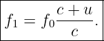
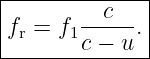
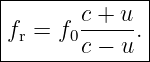
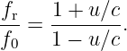
The Doppler effect is the change in observed frequency produced by relative motion between a
wave source and an observer.
For sound and other mechanical waves, one fact is essential:
The wave speed is measured relative to the material medium.
A moving observer changes the rate at which existing wavefronts are encountered.
A moving source changes the spacing of the wavefronts it emits.
Those are physically different mechanisms, although they combine into one compact
formula.
For one-dimensional propagation in the positive
direction, let:
- c be the wave speed relative to the medium,
- vs be the source velocity relative to the medium,
- vo be the observer velocity relative to the medium,
- positive velocities point in the propagation direction from source toward observer.
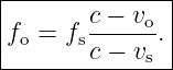
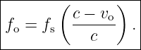
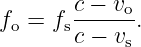
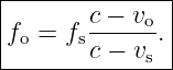
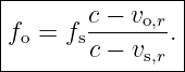
Then the classical Doppler formula is
With this convention:
- a source moving toward the observer has vs > 0 and raises the observed frequency,
- an observer moving toward the source has vo < 0 and raises the observed frequency.
The signs follow from geometry rather than from a memorized “approach means plus”
rule.
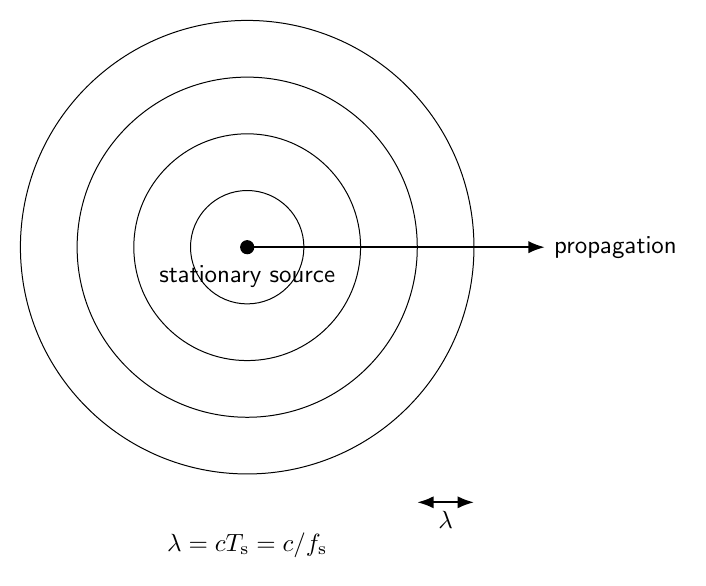
Figure 1. A stationary source emits equally spaced wavefronts into a stationary medium. The
source period fixes the spacing λ = c∕fs.
1 Stationary source and stationary observer
Let a stationary source emit at frequency
The source period is
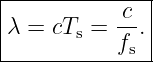
During one source period, a wavefront travels distance
Therefore the wavelength is
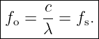
A stationary observer is crossed by wavefronts at rate
There is no Doppler shift.
2 Moving observer, stationary source
Now keep the source stationary and let the observer move.
The wavelength in the medium is unchanged:
The observer changes only the rate at which wavefronts are crossed.
For a wave propagating in the positive
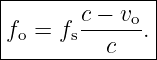
direction, the relative speed between the wavefronts and observer is
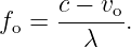
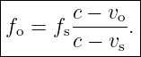
Therefore
Substituting
gives
If the observer moves toward the source,
so
The observed frequency rises.
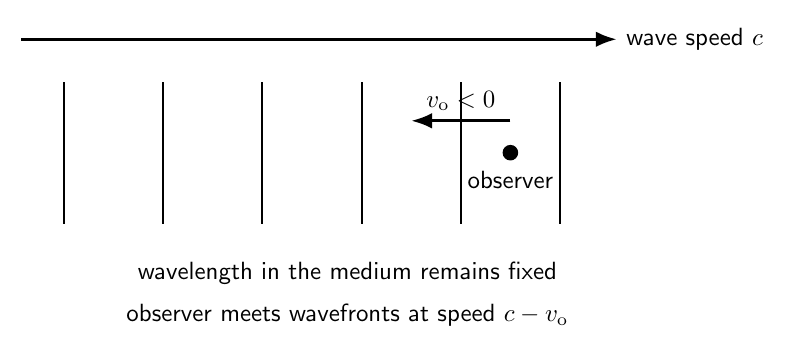
Figure 2. A moving observer does not change the wavelength already established in the medium.
Motion changes the wavefront encounter rate.
3 Example 1: observer moving toward a stationary source
Take
and let the observer move toward the source at
Since positive velocity points with the wave,
Then
| fo | = 1000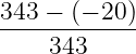 | (20)
|
| ≈ 1058.3 Hz. | (21) |
4 Moving source, stationary observer
Now let the observer remain stationary while the source moves in the propagation direction.
The source emits one crest, then moves before emitting the next crest.
During one source period,
the first crest moves forward distance
while the source moves forward distance
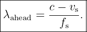
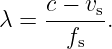
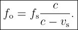
Therefore the wavelength ahead of the source is
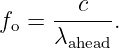
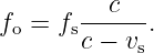
Equivalently,
The stationary observer receives wavefronts at rate
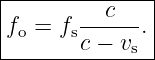
Hence
A source moving toward the observer has
so the wavelength is compressed and the frequency rises.
5 Wavefronts behind a moving source
Behind the source, the source moves away from previously emitted rearward wavefronts.
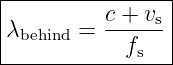
The rear wavelength is
when
denotes the source speed toward the forward observer.
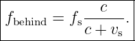
Thus a stationary observer behind the source measures
The moving source compresses wavefronts ahead and stretches them behind.
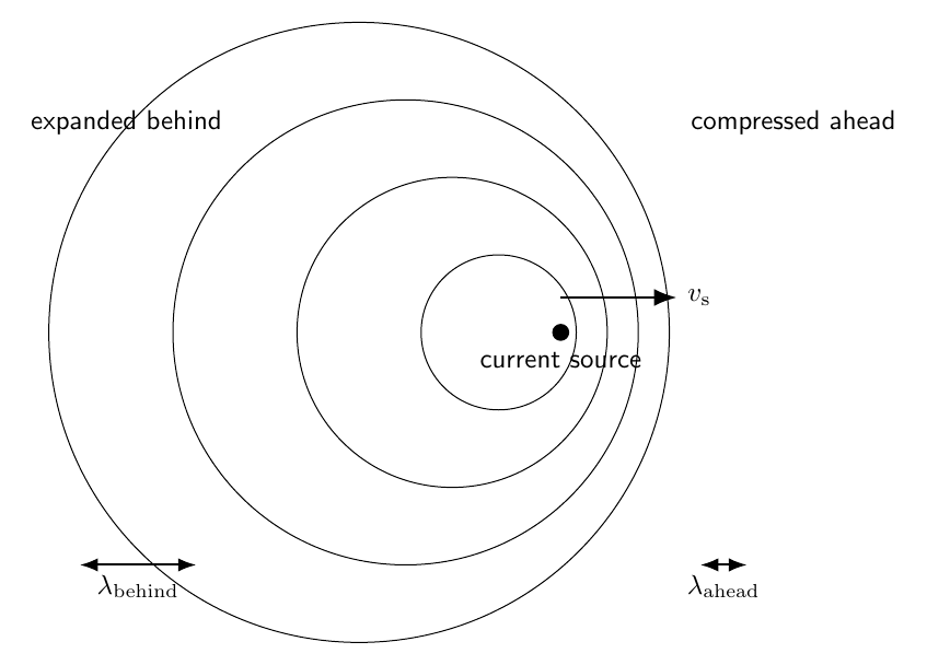
Figure 3. A subsonic source moving through the medium compresses wavefront spacing ahead and
expands it behind. The propagation speed relative to the medium remains c.
6 Example 2: source moving toward a stationary observer
Let
and
Then
| fo | = 1000 | (36)
|
| ≈ 1095.8 Hz. | (37) |
Behind the source,
| fbehind | = 1000 | (38)
|
| ≈ 919.6 Hz. | (39) |
7 Moving source and moving observer
The moving source first establishes the wavelength in the medium:
The moving observer then encounters those wavefronts at relative speed
Therefore
| fo | =  | (42)
|
| = 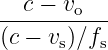 . | (43) |
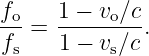
Thus
This equation should always be used together with a stated sign convention.
8 Sign convention
For the one-dimensional formula used here, the positive direction is the direction of wave
propagation from source toward observer.
Therefore:
- vs > 0: source moves toward observer,
- vs < 0: source moves away from observer,
- vo > 0: observer moves away from source,
- vo < 0: observer moves toward source.
This is summarized geometrically in Figure 4.
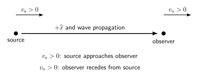
Figure 4. One-dimensional sign convention for a wave propagating from source to observer.
Positive velocity points with propagation. Source motion in the positive direction closes the
separation, while observer motion in the positive direction increases it.
9 Example 3: both source and observer moving
Let the source move toward the observer at
and let the observer move toward the source at
Then
For
and
| fo | = 1000 | (50)
|
| ≈ 1159.7 Hz. | (51) |
10 Why source and observer motion are not symmetric
For mechanical waves in a medium, source and observer velocities appear differently:
This asymmetry is physical.
The medium provides a preferred frame for propagation.
Observer motion changes encounter rate.
Source motion changes wavelength.
This is fundamentally different from the relativistic Doppler effect for light in vacuum, where no
material propagation medium defines a preferred frame.
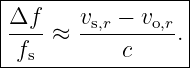
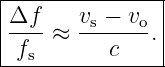
11 Low-speed approximation
Suppose
Then
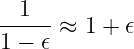
Using
for small
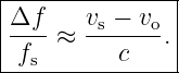
Therefore
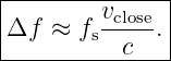
The leading-order shift depends on the closing velocity along the propagation direction.
12 Closing speed
Define
With the present sign convention,
means the source and observer are approaching.
Then at low speed,
This approximation is useful for quick estimates, but the exact classical expression should be used
when speeds are not very small compared with
13 Three-dimensional motion and radial velocity
Only the component of velocity along the propagation direction contributes directly to the
first-order Doppler shift.
Let
point along the acoustic ray from the source emission point toward the observer.
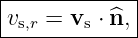
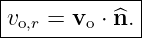
Define the radial velocity components
and
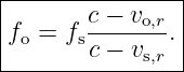
The corresponding classical ray formula is
For low speeds,
Transverse motion matters because it changes the line-of-sight direction with time, but the
instantaneous first-order shift is governed by radial components.
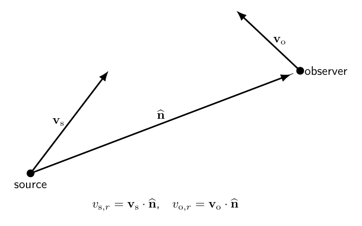
Figure 6. In multidimensional motion, project source and observer velocities onto the propagation
direction. The radial components determine the instantaneous classical Doppler shift along that
ray.
14 Passing source
Consider a source moving at constant speed
along a straight road.
Let the observer be a perpendicular distance
from the road.
Choose
when the source is at the point of closest approach.
The source position relative to the observer can be represented as
The source-observer distance is
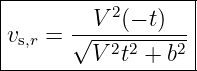
The source radial velocity toward the observer is
with the sign determined by the chosen propagation direction.
The important physical result is:
- before closest approach, the radial component is toward the observer and the received
frequency is elevated,
- at closest approach, the instantaneous radial component is zero,
- after closest approach, the radial component is away from the observer and the received
frequency is reduced.
In a realistic pass-by geometry, the frequency shift changes continuously rather than making the
discontinuous jump of an idealized one-dimensional crossing.
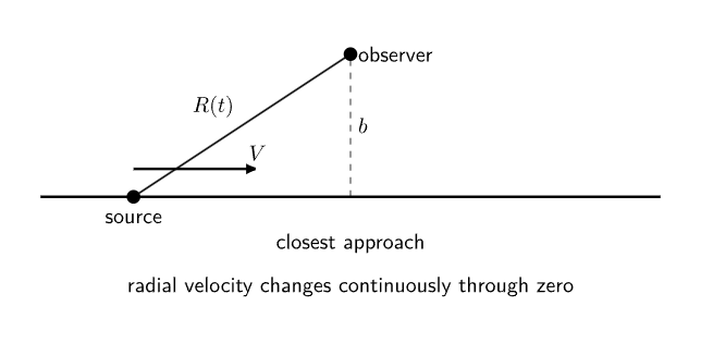
Figure 5. A source passing an observer at nonzero lateral distance has a radial velocity that
changes continuously from approaching to receding. At closest approach the instantaneous radial
component vanishes.
15 Doppler shift and beats
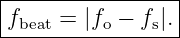
M06-13 developed the beat frequency
If one tone is an unshifted reference at
and the other is Doppler shifted to
their superposition produces beats at
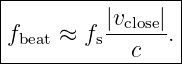
For small speeds,
Thus beat measurements can be used to infer a small velocity.
16 Example 4: velocity from an acoustic beat shift
A reference tone is
A Doppler-shifted return produces a beat frequency
For a one-way low-speed shift in air,
the corresponding closing speed is approximately
| vclose | ≈ c | (83)
|
| = 343 | (84)
|
| ≈ 3.43 m∕s. | (85) |
This example is one-way Doppler. Reflection introduces a second shift.
17 Reflection from a moving target
A wave reflected from a moving object undergoes two Doppler transformations.
First, the moving target acts as an observer.
Second, the target re-radiates or reflects the disturbance and therefore acts as a moving source for
the return path.
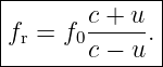
Consider a stationary transmitter and receiver at the same location.
Let a target move toward them at speed
The target first receives
For the reflected return, the approaching target acts as a moving source.
Therefore the receiver measures
Combining,
This is the classical double Doppler shift for an approaching reflector in this one-dimensional
geometry.
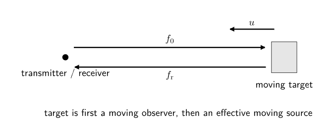
Figure 7. Reflection from a moving target produces two shifts. The target first receives the
incident wave as a moving observer, then returns it as an effective moving source.
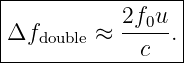
18 Low-speed double Doppler shift
For
Using the small-speed expansion,
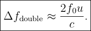
Thus
The factor of two is a consequence of the outgoing and return Doppler transformations.
19 Example 5: reflected acoustic Doppler shift
Take
and
The exact return frequency is
| fr | = 40000 | (97)
|
| ≈ 40469.2 Hz. | (98) |
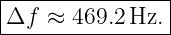
Thus
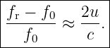
The low-speed approximation gives
| Δf | ≈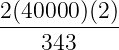 | (100)
|
| ≈ 466.5 Hz. | (101) |
The approximation is already close because
is small.
20 Effect of a moving medium
For sound, the velocity
is defined relative to the medium.
Therefore source and observer velocities in the classical formula should also be interpreted relative
to the same medium.
If the air itself moves relative to the ground, ground speeds cannot simply be inserted without
accounting for the medium velocity.
Let the medium velocity in the ground frame be
Then the source velocity relative to the medium is
and similarly
These medium-relative velocities belong in the acoustic Doppler formula.
21 Retarded emission time
When source motion is significant, the wave received at observation time
was emitted at an earlier time.
Call that time
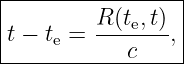
The propagation condition is
where
is the source-to-observer path length connecting the emission event to the reception
event.
This is the classical retarded-time condition.
For simple constant-velocity one-dimensional motion, it reduces to the formulas already
derived.
For arbitrary trajectories, solving the retarded geometry is the systematic approach.
22 The sonic limit
For a source moving toward a stationary observer,
As
the ideal formula predicts
This divergence signals the breakdown of the simple separated-wavefront picture.
Wavefronts emitted in the forward direction pile up.
At and above the wave speed, the geometry changes qualitatively.
The relevant physics becomes:
These topics are the natural continuation in M06-15.
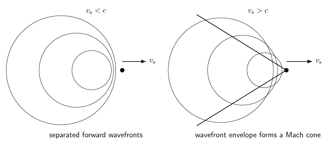
Figure 8. As a source approaches the wave speed, forward wavefront spacing collapses. At
supersonic speed the disturbance forms a Mach-cone geometry rather than an ordinary sequence
of separated forward wavefronts.
23 Why the classical formula cannot be used blindly at supersonic speed
If
the expression
becomes negative for the forward one-dimensional construction.
That does not mean the observer measures an ordinary negative frequency.
It means the assumptions behind the subsonic wavelength derivation no longer describe the
geometry.
The source overtakes its own wavefronts.
The disturbance must be analyzed using the envelope of wavefronts and shock propagation.
24 Common mistakes
- Treating the Doppler shift as a change in wave speed relative to the medium.
- Using the same physical argument for source motion and observer motion.
- Memorizing plus and minus signs without defining a coordinate direction.
- Forgetting that a moving observer does not change the wavelength already present in
the medium.
- Forgetting that a moving source changes the emitted wavelength.
- Assuming source and observer motion are symmetric for mechanical waves.
- Using ground-frame velocities when the medium itself is moving.
- Using total speed instead of the radial velocity component in multidimensional motion.
- Assuming transverse velocity produces the same first-order shift as radial velocity.
- Confusing source frequency with observed frequency.
- Applying the low-speed approximation when velocities are not small compared with c.
- Forgetting the second Doppler transformation in a moving-reflector problem.
- Missing the factor of two in the low-speed reflected Doppler shift.
- Assuming a passing source maintains a constant radial velocity.
- Extending the ordinary subsonic formula through the sonic limit without changing the
wavefront geometry.
25 Practice exercises
- Derive the moving-observer formula from the rate at which wavefronts cross the
observer.
- Derive the wavelength ahead of a moving source.
- Derive the wavelength behind a moving source.
- Combine the moving-source and moving-observer effects to obtain the one-dimensional
classical Doppler formula.
- Reproduce Examples 1 through 3 numerically.
- Derive the low-speed approximation for the one-dimensional Doppler shift.
- Rewrite the low-speed shift in terms of closing speed.
- Show why only radial velocity enters the first-order multidimensional shift.
- For a source passing an observer at lateral distance b, derive the source-observer
distance R(t).
- Use the Doppler-beat connection to estimate velocity from a specified beat frequency.
- Derive the exact double Doppler formula for an approaching reflector.
- Derive the factor-of-two low-speed approximation for reflected Doppler.
- Reproduce the 40 kHz reflected-shift example.
- Explain how a uniform wind changes which source and observer velocities belong in
the acoustic formula.
- Explain physically why the subsonic Doppler formula breaks down as source speed
approaches the wave speed.
26 Summary
For a stationary source and moving observer,
For a moving source and stationary observer,
Combining both effects,
At low speeds,
In multidimensional motion, use radial components:
For reflection from an approaching target,
At low speed,
The Doppler effect is therefore a direct consequence of wavefront timing, wavelength geometry,
observer encounter rate, and the propagation frame defined by the medium.
References
References
[1] PhysicsLibrary, M06-13, Beats, Interference, and Coherence.
[2] PhysicsLibrary, M06-11, Acoustic Waves, Sound Intensity, and Acoustic Impedance.
[3] PhysicsLibrary, M06-10, Fourier Analysis, Wave Packets, and Dispersion.
[4] A. P. French, Vibrations and Waves, W. W. Norton, 1971.
[5] L. E. Kinsler, A. R. Frey, A. B. Coppens, and J. V. Sanders, Fundamentals of
Acoustics, 4th ed., Wiley, 2000.