|
|
|
|||||||
From this one definition come the ideas of:
This companion is designed as deliberate practice. Every problem is stated first. Hints come next. Only after that are the complete worked solutions given. The goal is not speed. The goal is to make the projection mechanism so familiar that the Fourier coefficient derivations in FS04 and FS05 will feel like the same geometry in a trigonometric basis.
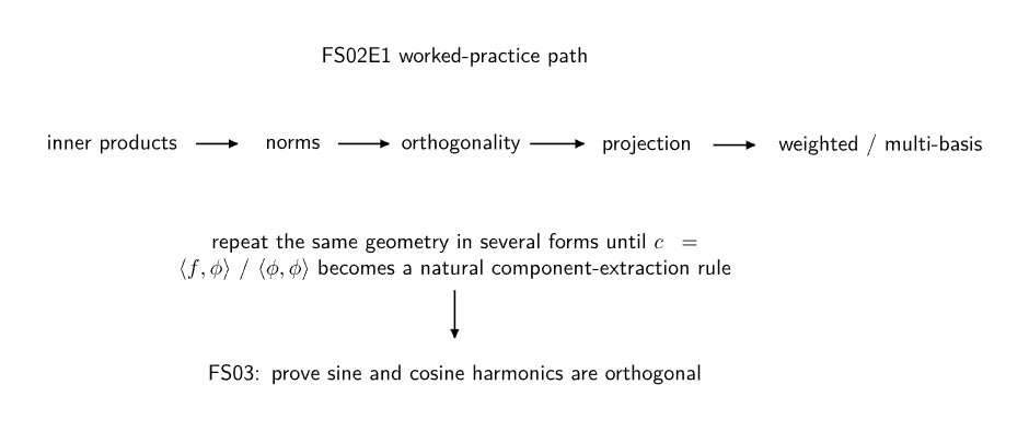
Figure 1. The exercise path. The problems begin with direct inner products and norms, then move through orthogonality and projection, and finish with weighted products and a preview of building an orthogonal basis.
1 Problems
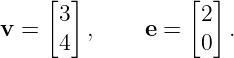
Problem 1: a vector projection warm-upLet
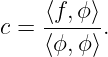
Find the scalar c such that
is the projection of v onto e. Then compute the residual
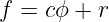
and verify
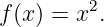
Problem 2: a basic function inner productOn [−1, 1], compute
Is the result positive, negative, or zero? What does that sign tell us geometrically?
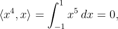
Problem 3: even and odd functionsOn [−1, 1], compute
Then explain why the answer could have been predicted before integrating.
Problem 4: the interval mattersFor the functions
compute the inner product on:
Are the functions orthogonal on both intervals?
Problem 5: norm and normalization of a constant functionOn [−L,L], where L > 0, let
Find:
Verify directly that
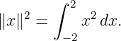
Problem 6: norm and normalization of xOn [−2, 2], compute
Then construct the normalized function
Problem 7: projection of x2 onto the constant functionOn [−1, 1], project
onto
Find the projection coefficient
Then write
and verify explicitly that
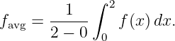
Problem 8: projection onto a constant equals an averageOn [0, 2], let
Project f onto the constant function 1. Then independently calculate the average value
Compare the two results.
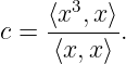
Problem 9: project x3 onto xOn [−2, 2], project
onto
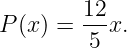
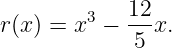
Find the coefficient c, the projected function cϕ, and the residual. Verify residual orthogonality directly.
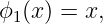
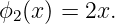
Problem 10: rescaling a basis functionOn [−1, 1], project
first onto
and then onto
Compare:
Explain why the coefficients differ even though the projected function is the same.
Problem 11: Pythagorean theorem for orthogonal functionsSuppose
Prove directly that
Do not skip the cross terms. Show explicitly why they vanish.
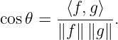
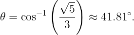
Problem 12: angle between two functionsOn [−1, 1], find the angle 𝜃 between
using
Give the exact value of cos 𝜃 and an approximate angle in degrees.
Problem 13: projection onto two orthogonal functionsOn [−1, 1], use the mutually orthogonal functions
Project
onto the span of these three functions. Find the three coefficients
Then simplify the projected function.
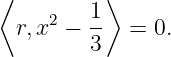
Problem 14: verify the three-function residualUse the projection found in Problem 13. Define
where P is the projection onto the three-function span. Verify separately that
and
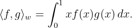
Problem 15: weighted projectionDefine the weighted inner product on [0, 1] by
Project
onto the constant function
Compare the result with the unweighted projection of x onto 1 on [0, 1].
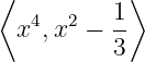
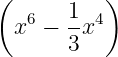
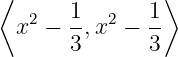
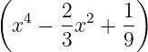
Problem 16: build a new orthogonal function by subtracting a projectionOn [−1, 1], begin with
and subtract its projection onto the constant function 1. Call the residual
Then:
This is a preview of the Gram-Schmidt idea.
2 Hints
3 Worked solutions
Solution 1: vector projection warm-upThe projection coefficient is
Compute the numerator:
Compute the denominator:
Thus
The projected vector is
The residual is
Now check orthogonality:
This is the finite-dimensional model for every projection calculation in the rest of the companion.
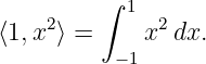
Solution 2: basic function inner productUse
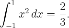
An antiderivative is
Therefore
The inner product is positive. In the geometric language of FS02, the angle between these two nonzero functions is acute rather than 90∘. They are not orthogonal.
Solution 3: even and odd functionsThe inner product is
An antiderivative is
Hence
The same answer could have been predicted immediately because:
Thus x and x2 are orthogonal on [−1, 1].
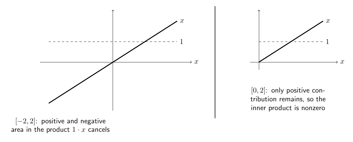
Solution 4: the interval mattersFirst use [−2, 2]:
Thus 1 and x are orthogonal on [−2, 2]. Now use [0, 2]:
This is not zero. Therefore the same two formulas are not orthogonal on [0, 2].
Figure 2. Orthogonality depends on the interval. On a symmetric interval the positive and negative contributions of the odd product cancel; on [0,2] there is no matching negative part.
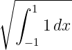
Solution 5: norm and normalization of a constant functionThe norm is
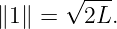
With f = 1,
Therefore
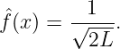
Normalize by dividing by the norm:
Check its norm:
Thus
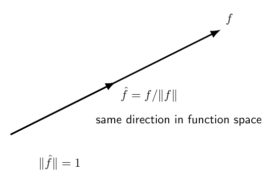
Figure 3. Normalization changes the length of a function-space vector without changing its direction. The normalized function has norm one.
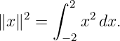
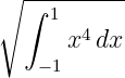
Solution 6: norm and normalization of xStart with
Because x2 is even,
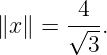
Hence
The normalized function is
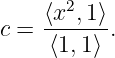
Solution 7: project x2 onto the constant functionUse
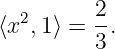
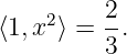
The numerator was already found in Problem 2:
The denominator is
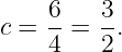
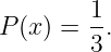
Therefore
Thus the projected function is
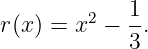
The residual is
Check the residual inner product with 1:
So the residual contains no remaining constant component.
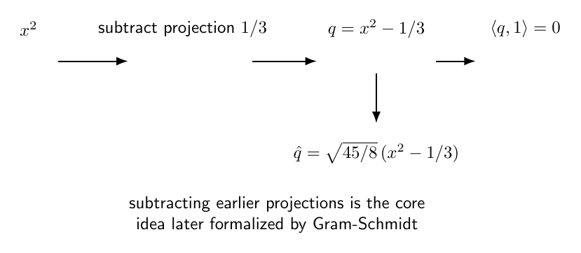
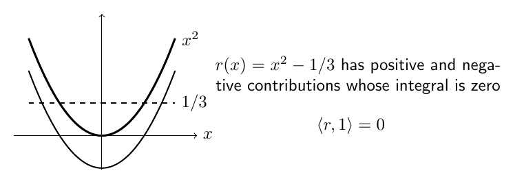
Figure 4. Projection splits x2 into a constant component 1∕3 and an orthogonal residual x2 − 1∕3. The residual has zero inner product with the constant basis function.
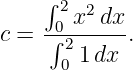
Solution 8: constant projection equals the averageProject x2 onto 1 on [0, 2]:
The numerator is
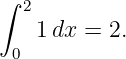
The denominator is
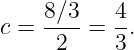
Therefore
Now calculate the average directly:
The two results are identical. Projection onto the constant function extracts the average value on the interval.
Solution 9: project x3 onto xUse
The numerator is
The denominator is
Therefore
The projection is
The residual is
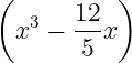
Now verify orthogonality:
Solution 10: rescaling the basis functionFirst project x3 onto x on [−1, 1]. The numerator is
The denominator is
Hence
Thus
Now use ϕ2 = 2x. The numerator is
The denominator is
Therefore
But the projected function is
Thus
The coefficient changed because the basis vector itself was rescaled. The one-dimensional subspace did not change. Projection depends on the subspace, while the numerical coefficient depends on how the basis vector is normalized.
Solution 11: Pythagorean theorem for orthogonal functionsStart from
Use linearity in both slots for real functions:
Orthogonality gives
Symmetry gives
Therefore both cross terms vanish:
This is exactly the function-space analogue of the ordinary Pythagorean theorem.
Solution 12: angle between 1 and x2The numerator is
The first norm is
The second norm is
Therefore
Thus
The angle is acute because the inner product is positive.
Solution 13: projection onto three orthogonal functionsWe use
Because the functions are mutually orthogonal, each coefficient can be calculated independently. For ϕ0:
For ϕ1 = x, symmetry gives
so
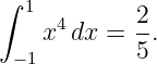
Now find c2. The numerator is
The denominator is
Therefore
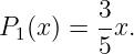
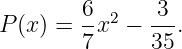
Thus the projection is
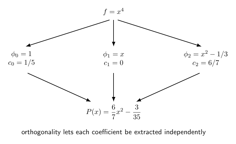
Figure 5. Projection onto several mutually orthogonal functions is obtained one component at a time. Orthogonality prevents the coefficient calculations from interfering with one another.
Solution 14: verify the three-function residualFrom Problem 13,
Therefore
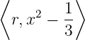
First check ⟨r, 1⟩:
Use denominator 35:
Next check ⟨r,x⟩. The residual is even and x is odd, so the product is odd:
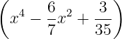
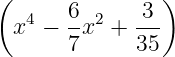
Finally check ⟨r,x2 − 1∕3⟩. A direct expansion gives
Therefore
Put everything over 105:
Thus the residual is orthogonal to every function in the projection subspace.
Solution 15: weighted projectionThe weighted projection coefficient is
The numerator is
The denominator is
Thus
For comparison, the ordinary unweighted projection is
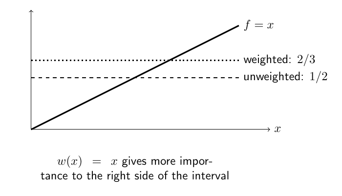
The weighted inner product gives greater importance to larger x, so the projected constant shifts upward from 1∕2 to 2∕3.
Figure 6. Weighting changes the geometry. With w(x) = x, the region near x = 1 contributes more strongly, so the best constant component of f(x) = x moves from 1∕2 to 2∕3.
Solution 16: subtracting a projection to make a new orthogonal functionFrom Problem 7, the projection of x2 onto the constant function is
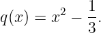
Therefore define
By construction,
We can verify this directly:
Now compute the norm squared:
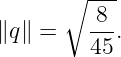
Thus
A normalized version is
Figure 7. Subtracting the projection of x2 onto the constant function produces x2 − 1∕3, which is orthogonal to 1. This is the essential idea behind Gram-Schmidt orthogonalization.
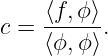
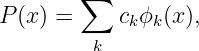
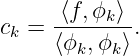
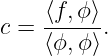
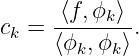
4 What these exercises are preparing us to doThe repeated pattern is now clear. Given a candidate basis function ϕ, the coefficient of the component of f along ϕ is
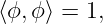
If the basis function is normalized,
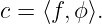
so
For several mutually orthogonal functions,
with
The next mathematical question is therefore unavoidable:
FS03 answers that question by deriving the required trigonometric integrals from first principles.
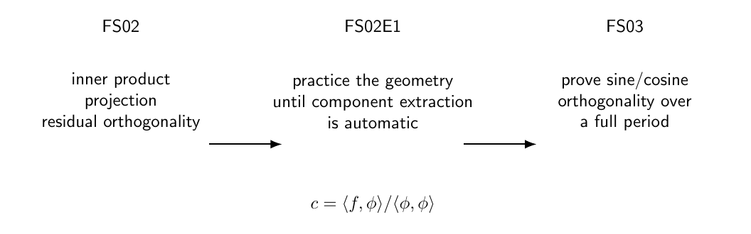
Figure 8. FS02E1 completes the projection toolkit. FS03 supplies the missing trigonometric fact: distinct sine and cosine harmonics are orthogonal over the appropriate interval.
5 Further practice
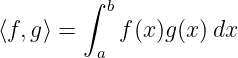
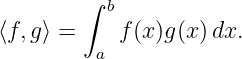
6 SummaryThe function inner product
turns many familiar vector ideas into tools for functions. A function is orthogonal to another when their inner product is zero. The norm is
Normalization gives
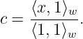
The projection coefficient of f onto a nonzero function ϕ is
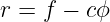
The residual
satisfies
For mutually orthogonal basis functions, the coefficients are extracted independently. A weighted inner product changes the geometry by changing how strongly different parts of the interval contribute. FS03 now specializes these general ideas to sine and cosine functions and proves their orthogonality one integral at a time.
References
References
"Function Inner-Product, Orthogonality, and Projection Exercises" is owned by bloftin.
This object's parent. Cross-references: FS03, period, function inner product, harmonics, theorem, vector, Weight, square, formula, vector projection, projection coefficient, normalized function, scalar, norms, Fourier coefficient, speed, weighted inner products, orthogonal functions, residual orthogonality, function norm, inner product, functions, FS02 There is 1 reference to this object. This is version 1 of Function Inner-Product, Orthogonality, and Projection Exercises, born on 2026-10-22. Object id is 1520, canonical name is FunctionInnerProductOrthogonalityAndProjectionExercises. Accessed 12 times total. Classification:
|
|
|
|
Pending Errata and AddendaNone.
|
DiscussionNo messages.
|
Interact |





























 (2









 (2)












 (2

















 +
 (2)

 +


 +


 +






 +
 (2)

 +


 +


 +






 +


 (2)

 +


 +