Electromagnetic Waves, Antennas, and RF: End-to-End RF and GNSS Link-Budget
Synthesis
The preceding articles developed the pieces of a radio link separately. EM24 introduced antenna
gain, EIRP, and effective aperture; EM25 derived Friis and free-space path loss; EM26 developed
thermal noise, system noise temperature, G∕T, and C∕N0; and EM27 added received interference
and receiver degradation. EM28 now assembles those pieces into one consistent end-to-end
calculation [1, 2, 3, 4, 5].
The basic engineering chain is
- Pt
- EIRP
- path loss
- C
- G∕T
- C∕N0
- C∕N
- interference margin
The purpose is not merely to collect formulas. A reliable link budget requires every term to refer to
a stated physical reference plane, to use compatible units, and to avoid counting the same gain or
loss twice.
1 The complete signal chain
Consider a transmitter and receiver separated by range r. The transmitter begins with power Pt at
some stated reference plane. A transmit feeder or implementation loss Lt reduces the power before
the antenna, while the antenna gain Gt redistributes the radiated power in angle. The resulting
equivalent isotropically radiated power is
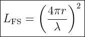
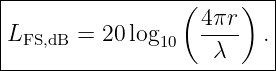
The wave then experiences propagation loss. For ideal free space,
and
Additional terms may include atmospheric absorption, rain attenuation, polarization
mismatch, pointing loss, radome loss, ionospheric or scintillation allowances, and other
modeled impairments. We collect these as Lother when their detailed separation is not
needed.
At the receiver, the antenna gain in the desired-signal direction is Gr. The received carrier power
at the stated receiver reference plane is therefore
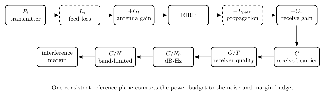
Figure. End-to-end link-budget chain. Each stage converts one physical quantity into the
next; the dB signs follow whether the stage adds gain or removes power.
2 Why the reference plane matters
The expression above is only correct if the terms are defined consistently. For example, if EIRP
already includes transmit feeder loss, that same feeder loss must not be subtracted again. Likewise,
if a quoted receive G∕T already includes a lossy cable ahead of the LNA through the
system-noise-temperature calculation, that cable loss must not also be independently subtracted
from C∕N0 unless the reference plane is changed consistently.
A useful receiver reference plane is the antenna terminal. At that plane,
- Gr is the receiving antenna gain toward the transmitter;
- Tsys contains antenna noise plus all receiver noise referred back to that terminal;
- preamplifier cable or filter losses are included in Tsys through their equivalent noise
temperature when appropriate.
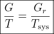
The system figure of merit is then
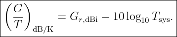
or, in logarithmic form,
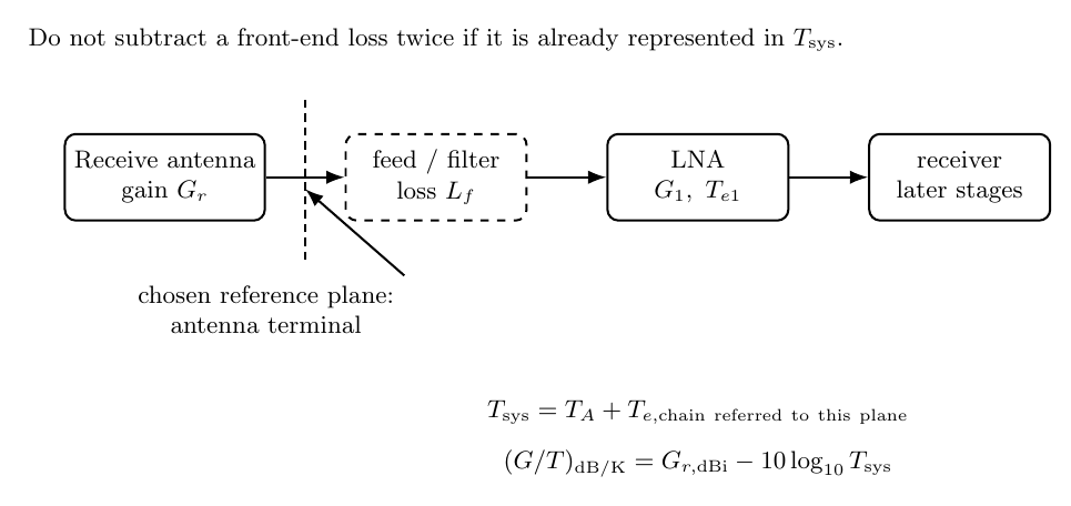
Figure. Receiver reference-plane bookkeeping. Receive gain and system noise temperature
must be referred to compatible planes before they are combined as G∕T.
3 From received carrier power to C∕N0
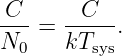
EM26 established the thermal-noise density
where
Thus
In dB units,
 dB−Hz dB−Hz | = CdBW − 10 log 10k − 10 log 10Tsys. | (10) |
Since
we obtain
Now substitute
Grouping Gr − 10 log 10Tsys gives the compact end-to-end result
This is one of the most useful equations in satellite and GNSS link analysis. It combines
transmitter strength, propagation, receiver antenna gain, and receiver thermal performance into
one bandwidth-independent carrier-quality metric.
4 From C∕N0 to finite-bandwidth C∕N
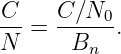
For an effective noise bandwidth Bn,
Therefore
In logarithmic form,
This distinction is essential for spread-spectrum systems. A GNSS signal may have negative
pre-correlation C∕N across a wide RF bandwidth while still possessing a useful C∕N0 because the
receiver later exploits known signal structure and processing gain.
5 A complete RF link-budget table
An end-to-end dB budget can be organized so that every row has a sign and a physical
interpretation:
|
|
|
| Quantity | Symbol | Sign in budget |
|
|
|
| Transmit power | Pt | + |
| Transmit feed loss | Lt | − |
| Transmit antenna gain | Gt | + |
| Free-space path loss | LFS | − |
| Other propagation / polarization losses | Lother | − |
| Receive antenna gain | Gr | + |
| Thermal term | 10 log 10Tsys | − in C∕N0 |
| Boltzmann conversion | −10 log 10k | +228.60 |
| Receiver bandwidth | 10 log 10Bn | − in C∕N |
|
|
|
A good practical check is to calculate the link in two independent ways:
- compute the received carrier C first and then subtract N0;
- compute C∕N0 directly using EIRP, path loss, and G∕T.
The two results should agree when the reference planes are consistent.
6 Worked example 1: complete microwave-style RF link
Suppose an RF link has
| Pt | = 10 W = 10 dBW, | (18)
|
| Lt | = 1.0 dB, | (19)
|
| Gt | = 24 dBi, | (20)
|
| f | = 5.8 GHz, | (21)
|
| r | = 5.0 km, | (22)
|
| Lother | = 2.0 dB, | (23)
|
| Gr | = 20 dBi, | (24)
|
| Tsys | = 500 K, | (25)
|
| Bn | = 1.0 MHz. | (26) |
The EIRP is
The free-space path loss is approximately
Thus
| C | = 33 − 121.69 − 2 + 20 | (29)
|
| ≈−70.69 dBW. | (30) |
The system noise density is
| N0 | = 10 log 10(kTsys) | (31)
|
| ≈−201.60 dBW/Hz. | (32) |
Hence
For Bn = 1 MHz,
This example is intentionally a strong terrestrial link; its purpose is to verify the bookkeeping
before moving to the much weaker received powers typical of satellite navigation.
7 Worked example 2: GNSS-style end-to-end synthesis
Consider an illustrative L1-like link with
| f | = 1.57542 GHz, | (35)
|
| r | = 20,200 km, | (36)
|
| EIRP | = 27.0 dBW, | (37)
|
| Lother | = 2.0 dB, | (38)
|
| Gr | = 2.0 dBi, | (39)
|
| Tsys | = 400 K, | (40)
|
| Bn | = 2.0 MHz. | (41) |
These values are illustrative for learning the link-budget method; they are not intended as a
specification for a particular GNSS spacecraft or receiver.
The free-space path loss is
The received carrier at the antenna-terminal reference plane is
| C | = 27.0 − 182.50 − 2.0 + 2.0 | (43)
|
| ≈−155.50 dBW . | (44) |
The receiver figure of merit is
| G∕T | = 2.0 − 10 log 10(400) | (45)
|
| ≈−24.02 dB/K . | (46) |
Using the direct end-to-end formula,
| C∕N0 | = 27.0 − 182.50 − 2.0 − 24.02 + 228.60 | (47)
|
| ≈ 47.08 dB-Hz . | (48) |
The same result follows from the carrier power. At 400 K,
so
Across a 2 MHz front-end bandwidth,
| C∕N | = 47.08 − 10 log 10(2 × 10⁶) | (51)
|
| ≈−15.93 dB . | (52) |
The negative wideband C∕N does not contradict useful GNSS reception; it simply shows why
correlation and signal processing are necessary.
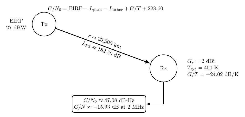
Figure. GNSS-style synthesis. A very large propagation loss can still yield a usable C∕N0
when the transmitter EIRP and receiver G∕T are combined consistently.
8 Adding received interference
Suppose an interfering signal produces received power J at the same receiver reference plane. The
first useful ratio is
If desired and interfering signals are computed as separate links,
| CdBW | = EIRPs − Ls + Gr,s, | (54)
|
| JdBW | = EIRPj − Lj + Gr,j, | (55) |
where all loss terms are expressed positively and subtracted. Therefore
The receiving antenna generally has different directional gains toward the desired and interfering
sources. That angular discrimination belongs explicitly in the link budget.
For a broadband noise-like interferer, it is often more useful to work with interference spectral
density J0. Define
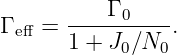
The effective carrier-to-noise-plus-interference density is then
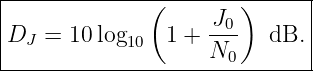
Thus the interference degradation is
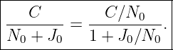
The degraded density ratio is simply
9 Interference margin from a required C∕N0
Suppose the no-interference link provides
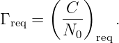
and the receiver requires at least
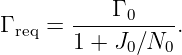
With noise-like interference density J0,
At the threshold of acceptable performance,
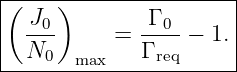
Solving for allowable interference gives
If the available C∕N0 margin is
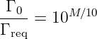
then
and therefore
This is a receiver-side robustness margin. It states how much additional noise-like interference
density can be tolerated at the chosen reference plane before the specified C∕N0 threshold is
reached.
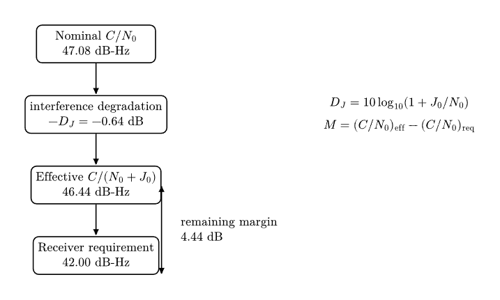
Figure. Link-margin bookkeeping. A nominal C∕N0 is reduced by modeled degradations; the
remaining separation from the receiver requirement is the available margin.
10 Worked example 3: interference margin on the GNSS-style link
Continue the illustrative GNSS-style link with
Assume a receiver requirement of
The no-interference margin is
The largest noise-like interference density ratio consistent with that threshold is
| (J0∕N0)max | = 105.08∕10 − 1 | (72)
|
| ≈ 2.22, | (73) |
so
At 400 K,
so the corresponding receiver-plane interference-density threshold is
Now suppose the actual admitted noise-like interference density is
Its degradation is
| DJ | = 10 log 10(1 + 10−8∕10) | (78)
|
| ≈ 0.64 dB . | (79) |
The effective density ratio becomes
The remaining margin above the 42 dB-Hz requirement is therefore
Over the same 2 MHz bandwidth, thermal noise is
and the interference power is
Since the carrier is −155.50 dBW,
This is an instructive result: the admitted interference can be several decibels stronger than the
desired spread-spectrum carrier while still remaining well below the total thermal noise in a wide
front-end bandwidth. Consequently J∕S alone does not determine receiver degradation;
bandwidth, spectrum, correlation, and receiver architecture matter.
11 Link margin, implementation margin, and uncertainty
A link budget often contains several distinct margins. They should not be merged blindly.
Propagation or availability margin
This allowance covers fading, atmospheric variability, pointing uncertainty, or other propagation
effects not represented by the nominal path model.
Receiver implementation loss
A practical receiver may perform worse than an ideal detector by an implementation loss Limpl.
This can be handled either by increasing the required C∕N0 threshold or by subtracting a clearly
labeled implementation allowance from the available margin. It should not be counted both
ways.
Interference margin
This is the room between the nominal thermal-noise-limited operating point and the requirement
that may be consumed by additional interference. For noise-like interference, the nonlinear
relation
should be used rather than simply subtracting J0∕N0 in dB.
Model uncertainty
Antenna pattern error, cable-loss uncertainty, temperature uncertainty, and calibration error may
be carried as explicit uncertainty terms. A conservative design should state whether such
terms are deterministic worst-case values, statistical standard deviations, or engineering
reserves.
12 Common bookkeeping failures
Several errors recur in RF and GNSS link calculations.
- Double-counting antenna gain. If EIRP already contains Gt, do not add Gt again.
- Double-counting receive loss. A cable loss incorporated into Tsys or a quoted G∕T
should not also be subtracted independently without changing the reference plane.
- Mixing dBW and dBm. They differ by exactly 30 dB:
- Confusing C∕N0 with C∕N. The former is in dB-Hz; the latter depends explicitly on
bandwidth.
- Adding powers directly in dB. Independent noise and interference powers must be added
in linear units before conversion back to decibels.
- Using J∕S as a complete receiver metric. It does not by itself include receiver
bandwidth, spectral overlap, filtering, correlation, AGC behavior, or nonlinear front-end
effects.
- Using a scalar margin without a requirement. A margin is meaningful only relative to
a stated threshold and reference condition.
13 Compact end-to-end workflow
A practical calculation can follow the sequence
| EIRP | = Pt − Lt + Gt, | (87)
|
| C | = EIRP − Lpath − Lother + Gr, | (88)
|
| G∕T | = Gr − 10 log 10Tsys, | (89)
|
| C∕N0 | = EIRP − Lpath − Lother + G∕T + 228.60, | (90)
|
| C∕N | = C∕N0 − 10 log 10Bn, | (91)
|
| DJ | = 10 log 10(1 + J0∕N0), | (92)
|
| (C∕(N0 + J0))dB−Hz | = (C∕N0)dB−Hz − DJ, | (93)
|
| M | = (C∕(N0 + J0))dB−Hz − (C∕N0)req,dB−Hz. | (94) |
Every line should be annotated with its reference plane and assumptions. That discipline is more
important than any individual numerical formula.
14 Summary
EM28 combines the preceding RF topics into a single end-to-end link model. The transmitter is
summarized by
propagation by
and the receiver by
These combine to give
with C∕N0 in dB-Hz when the other terms use the stated logarithmic units.
Finite bandwidth gives
while additive noise-like interference produces
Finally, the receiver-side interference allowance associated with a C∕N0 margin M is
The complete physical chain is therefore
This synthesis provides the foundation for detailed satellite-navigation receiver performance
studies, measurement-based link validation, and later treatments of acquisition, tracking,
processing gain, and integrity.
References
[1] H. T. Friis, “A Note on a Simple Transmission Formula,” Proceedings of the IRE, vol.
34, no. 5, pp. 254–256, 1946.
[2] D. M. Pozar, Microwave Engineering, 4th ed., Wiley, 2012.
[3] C. A. Balanis, Antenna Theory: Analysis and Design, 4th ed., Wiley, 2016.
[4] E. D. Kaplan and C. J. Hegarty, eds., Understanding GPS/GNSS: Principles and
Applications, 3rd ed., Artech House, 2017.
[5] J. W. Betz, Engineering Satellite-Based Navigation and Timing: Global Navigation
Satellite Systems, Signals, and Receivers, Wiley-IEEE Press, 2016.
[6] P. Misra and P. Enge, Global Positioning System: Signals, Measurements, and
Performance, 2nd ed., Ganga-Jamuna Press, 2011.