|
|
|
|||||||
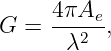
and
Unless a problem states otherwise, gains are power ratios, propagation is in free space, polarization is matched, the receiver is conjugately matched, and quoted electric-field phasor magnitudes are peak amplitudes.
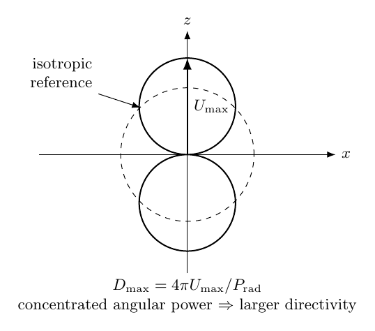
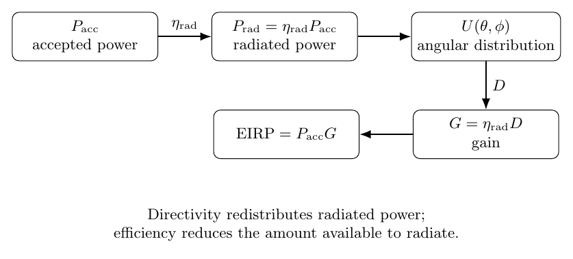
Figure. The antenna calculation chain begins with an angular power distribution and ends with directional gain. Efficiency changes gain without changing the idealized normalized pattern.
Part I: Exercises
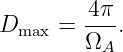
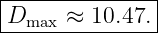
Exercise 1: radiation intensity and directivity of a Hertzian-type patternAn antenna has radiation intensity
independent of ϕ. Find (a) the total radiated power, (b) the maximum directivity, and (c) the maximum directivity in dBi.
Exercise 2: beam solid angleAn antenna has beam solid angle
Find its maximum directivity and maximum directivity in dBi.
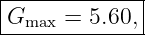
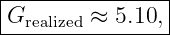
Exercise 3: radiation efficiency and gainAn antenna accepts 20.0 W at its terminals and radiates 14.0 W. In the direction of peak radiation its directivity is Dmax = 8.00. Find (a) radiation efficiency, (b) dissipative loss power, (c) peak gain, and (d) peak gain in dBi.
Exercise 4: realized gain and antenna mismatchThe antenna of Exercise 3 has an input reflection coefficient with magnitude
Using
find the realized gain in linear form and dBi. Also find the mismatch loss in dB.
Exercise 5: EIRP, power density, and electric-field strengthA transmitter supplies 10.0 W of accepted power to an antenna having gain G = 12.0 in the observation direction. At a range of 2.00 km, find (a) EIRP, (b) far-field power density, and (c) RMS electric-field magnitude in free space.
Exercise 6: dB link-budget bookkeeping at the transmitting antennaA transmitter output is 37.0 dBm. A feed cable introduces 2.0 dB loss before an antenna whose gain is 8.0 dBi. Find the EIRP in dBm and watts. State clearly which power reaches the antenna terminals.
Figure. Directivity describes angular redistribution of radiated power. Radiation efficiency converts accepted power to radiated power; gain combines the two; EIRP combines gain with accepted transmitter power.
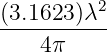
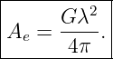
Exercise 7: effective aperture at GPS L1For GPS L1,
Find the maximum effective aperture of (a) an ideal 0 dBi antenna and (b) an antenna with 5.00 dBi gain.
Exercise 8: received power from incident power densityAt 1.20 GHz a receiving antenna has gain 6.00 dBi in the source direction. A matched-polarization plane wave arrives with power density
Find the antenna effective aperture and the maximum available receive power in watts and dBm.
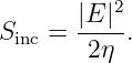
Exercise 9: derive the Hertzian-dipole effective apertureFor a Hertzian dipole oriented with the incident electric field, use
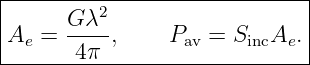
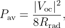
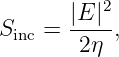
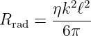
and
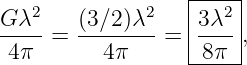
to derive Ae = Pav∕Sinc. Show that the result is identical to Gλ2∕(4π) for an ideal Hertzian dipole.
Exercise 10: polarization mismatchTwo linearly polarized antennas have polarization axes separated by 35.0∘. Find the polarization loss factor and polarization loss in dB. If the received power would be −90.0 dBm under matched polarization, what power is available after polarization mismatch alone?
Exercise 11: physical aperture, aperture efficiency, and dish gainA circular aperture antenna has diameter
aperture efficiency ηap = 0.650, and operates at 10.0 GHz. Find its physical area, effective aperture, gain, and gain in dBi.
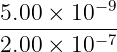
Exercise 12: infer gain from measured effective apertureA receiving antenna intercepts
from an incident power density
at 2.00 GHz. Find Ae, then infer antenna gain in linear units and dBi.
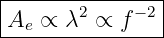
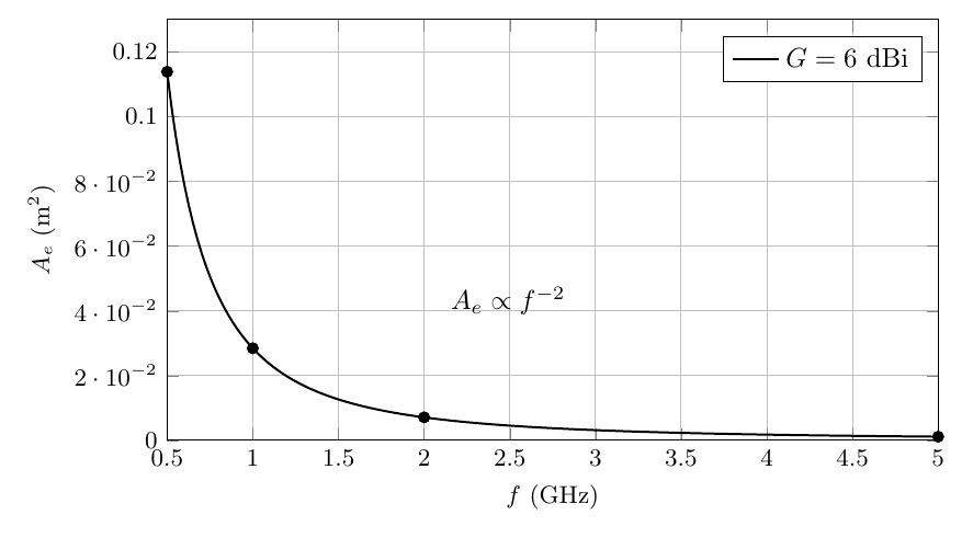
Figure. At fixed gain, effective aperture scales as λ2 and therefore as 1∕f2. The antenna can have the same dimensionless gain at two frequencies while intercepting different effective areas.
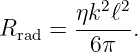
Exercise 13: numerical check of the Hertzian-dipole aperture derivationAt 300 MHz, a Hertzian dipole has length ℓ = λ∕50. A matched-polarization plane wave has peak electric-field phasor magnitude |E| = 1.00 V/m. Calculate (a) Rrad, (b) open-circuit voltage, (c) maximum available receive power, (d) incident time-average power density, and (e) effective aperture. Verify the result against
Exercise 14: frequency scaling of effective apertureAn antenna has constant gain G = 10.0 at both 1.00 GHz and 2.00 GHz. Find the effective aperture at each frequency and their ratio. Explain why a fixed gain does not imply a fixed effective area.
Exercise 15: transmit-to-receive bridgeA transmitter has accepted antenna power Pt = 2.00 W and directional gain Gt = 10.0. A receiver 10.0 km away has gain Gr = 4.00 toward the transmitter. The frequency is 1.00 GHz. Compute the received power in two stages:
Finally combine the expressions algebraically and identify the Friis form that EM25 will derive in detail.
Exercise 16: Julia sweep of gain, effective aperture, and EIRPWrite a Julia program that
State the expected scaling before writing the code.
Part II: Complete Worked Solutions
Solution 1: radiation intensity and directivityThe radiated power is
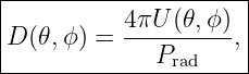
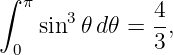
Using
we obtain
The maximum radiation intensity occurs at 𝜃 = 90∘:
Therefore
Thus
In dBi,
This reproduces the ideal Hertzian-dipole directivity derived in EM23 and EM24.
Solution 2: beam solid angleThe beam-solid-angle identity is
Hence
Therefore
In logarithmic form,
A small beam solid angle corresponds to high directivity because the radiated power is concentrated into a smaller set of directions.
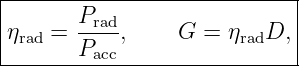
Solution 3: radiation efficiency and gainRadiation efficiency is
Thus
The dissipative loss is
Gain combines efficiency and directivity:
Therefore
and
Directivity describes how the radiated power is shaped; gain additionally remembers that 30% of accepted power was dissipated rather than radiated.
Solution 4: realized gain and mismatchThe mismatch efficiency is
Hence
Thus
with
The mismatch factor itself corresponds to
Thus the mismatch loss magnitude is
Solution 5: EIRP, power density, and field strengthThe EIRP is
Thus
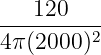
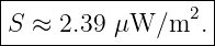
At r = 2000 m,
Therefore
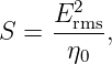
For a free-space plane wave,
so
Hence
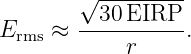
Using η0 ≈ 120π Ω gives the familiar equivalent form
Solution 6: dB transmitter bookkeepingThe cable reduces the 37.0 dBm transmitter output to
Thus 35.0 dBm, not 37.0 dBm, reaches the antenna terminals. Adding antenna gain,
Therefore
Converting to watts,
Hence
The result is an isotropic-equivalent directional power, not the actual total power radiated in all directions.
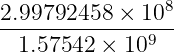
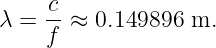
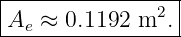
Solution 7: effective aperture at GPS L1The wavelength is
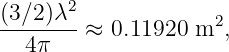
For 0 dBi, G = 1, so
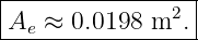
Thus
For 5.00 dBi,
Therefore
Hence
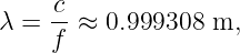
Solution 8: received power from incident power densityThe wavelength is
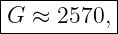
The linear gain corresponding to 6.00 dBi is
Hence
Thus
The maximum available receive power is
Therefore
In dBm,
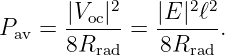
Solution 9: derive the Hertzian-dipole effective apertureStart from the available receive power under conjugate match:
The incident time-average power density is
Therefore
Now substitute
Then
Using
we get
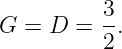
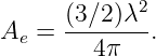
For an ideal Hertzian dipole,
Therefore
which is the same result. The receive calculation and the transmit directivity therefore meet at the reciprocity relation
Solution 10: polarization mismatchFor two linear polarizations separated by angle Δα,
Thus
Therefore
The loss magnitude is
Hence the received power becomes
This is a receive-orientation loss, not a free-space propagation loss.
Solution 11: physical aperture, aperture efficiency, and dish gainThe physical aperture area is
Thus
The effective aperture is
At 10.0 GHz,
Therefore
Hence
with
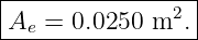
Solution 12: infer gain from measured effective apertureFirst,
Thus
At 2.00 GHz,
Using
we obtain
In dBi,
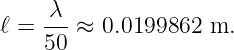
Solution 13: numerical Hertzian-dipole aperture checkAt 300 MHz,
so
Using the exact vacuum-impedance form,
Thus
The peak open-circuit phasor voltage is
The maximum available power is
The incident time-average power density is
Therefore
Thus
The gain relation predicts
which agrees exactly apart from rounding.
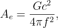
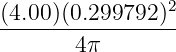
Solution 14: frequency scaling of effective apertureFor fixed gain,
so
At 1.00 GHz,
At 2.00 GHz,
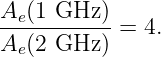
Their ratio is
Doubling frequency halves wavelength, and squaring that change reduces effective aperture by a factor of four. Gain is dimensionless directional performance; effective aperture is an area and therefore retains the wavelength scale.
Solution 15: transmit-to-receive bridgeThe wavelength at 1.00 GHz is
The transmitter EIRP in the receiver direction is
At r = 10.0 km,
The receiver effective aperture is
Thus
Therefore
Combining the two stages algebraically gives
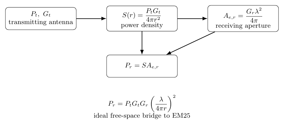
This is the ideal free-space Friis transmission relation. EM25 will separate this result into antenna terms, propagation loss, and practical link losses.
Figure. The two-step electromagnetic interpretation of Friis: transmitting gain produces power density at the receiver, and receiving effective aperture converts that density into available power.
Solution 16: Julia sweepBefore computation, the expected scalings are
for fixed gain, and
for fixed accepted power. A direct Julia implementation is provided with this article as
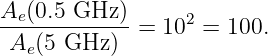
EM24E1_gain_aperture_sweep.jl. Its core calculations are c = 299792458.0 Pacc = 5.0 Gfixed_dBi = 6.0 Gfixed = 10.0^(Gfixed_dBi/10.0) f = range(0.5e9, 5.0e9, length=200) lambda = c ./ f Ae = Gfixed .* lambda.^2 ./ (4*pi) ratio_numeric = Ae[1] / Ae[end] ratio_expected = (f[end] / f[1])^2 gain_dBi = 0.0:1.0:15.0 gain = 10.0 .^ (gain_dBi ./ 10.0) EIRP = Pacc .* gain r = 1000.0 S = EIRP ./ (4*pi*r^2) Because the frequency changes by a factor of ten, the endpoint effective-aperture ratio should be
The gain sweep should increase EIRP and far-field power density by the same linear gain factor.
What EM24E1 adds to the seriesEM24 established the conceptual bridge from radiation pattern to receive aperture. EM24E1 makes that bridge operational through direct calculations and inverse problems. The complete chain is now
The final worked problem already exposes the ideal Friis equation. EM25 can therefore focus on the physical meaning of free-space path loss, logarithmic link budgets, system losses, and the assumptions under which Friis is valid.
References
References
[1] Constantine A. Balanis, Antenna Theory: Analysis and Design, 4th ed., Wiley, 2016. [2] Warren L. Stutzman and Gary A. Thiele, Antenna Theory and Design, 3rd ed., Wiley, 2012. [3] John D. Kraus and Ronald J. Marhefka, Antennas for All Applications, 3rd ed., McGraw-Hill, 2002. [4] IEEE, IEEE Standard for Definitions of Terms for Antennas, IEEE Std 145-2013, 2014. [5] David J. Griffiths, Introduction to Electrodynamics, 4th ed., Cambridge University Press, 2017. "Electromagnetic Waves, Antennas, and RF: Antenna Directivity, Radiation Efficiency, Gain, EIRP, and Effective Aperture - Exercises and Complete Worked Solutions" is owned by bloftin.
This object's parent. Cross-references: system, free-space path loss, computation, linear polarizations, identity, EM23, program, frequency, units, antenna gain, polarization loss factor, electric field, realized gain, radiation efficiency, beam solid angle, amplitudes, magnitudes, relations, EM25, Friis transmission equation, effective aperture, power, radiation, EM24 This is version 1 of Electromagnetic Waves, Antennas, and RF: Antenna Directivity, Radiation Efficiency, Gain, EIRP, and Effective Aperture - Exercises and Complete Worked Solutions, born on 2026-10-10. Object id is 1454, canonical name is ElectromagneticWavesAntennasAndRFAntennaDirectivityRadiationEfficiencyGainEIRPAndEffectiveApertureExercisesAndCompleteWorkedSolutions. Accessed 30 times total. Classification:
|
|
|
|
Pending Errata and AddendaNone.
|
DiscussionNo messages.
|
Interact |
![[parent]](https://images.physicslibrary.org/images/uparrow.png)














 = 1
= 1