Observational Foundations for Binary Stars
Binary star astrophysics begins with observables, not orbital elements.
A detector records photons. Those photons are converted into quantities such as
Those observables must then be calibrated, assigned uncertainties, and attached to a reference
system before they can be used to infer stellar or orbital parameters.
For binary stars this bookkeeping is especially important because two stars can contribute to the
same image pixel, spectrum, or photometric aperture.
The central observational chain is

Figure 1. Binary star inference begins with calibrated observables. Detector counts become fluxes,
magnitudes, spectra, positions, and times before they are interpreted with a physical model.
1 What a detector measures
An astronomical detector does not directly measure stellar mass, radius, luminosity, or orbital
inclination.
A photon-counting detector measures a number of detected photoelectrons or counts over an
exposure.
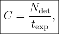
A simplified count rate can be written
where Ndet is the number of detected photoelectrons and texp is the exposure time.
The relationship between incident energy flux and detector counts depends on
- telescope collecting area,
- filter transmission,
- detector quantum efficiency,
- atmospheric transmission for ground-based data,
- wavelength dependence of the instrument,
- aperture and background subtraction.
Calibration is the process that connects instrumental measurements to physically interpretable
observables.
2 Luminosity and flux
The luminosity L of a star is the total power it radiates.
Its SI unit is
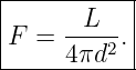
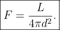
If radiation is emitted isotropically, the bolometric flux measured at distance d is
Flux has SI units
This inverse-square law is fundamental, but an astronomical catalog often reports a passband flux
rather than a bolometric flux.
The measured flux therefore depends on the instrument and wavelength range.
3 Bandpass flux
A real detector has a wavelength-dependent response.
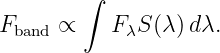
If Fλ is the spectral flux density and S(λ) is the total instrumental response, a simplified bandpass
measurement has the structure
The precise calibration depends on whether one works with energy-weighted or photon-weighted
response and on the adopted magnitude system.
The important point is
A V magnitude, Gaia G magnitude, and TESS magnitude are not interchangeable.
4 The astronomical magnitude scale
Magnitudes encode flux ratios logarithmically.
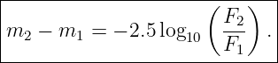
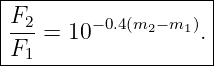
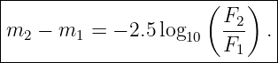
For two measurements in the same calibrated passband,
Equivalently,
A smaller magnitude corresponds to a larger flux.
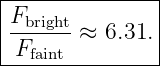
A difference of five magnitudes corresponds to a factor of one hundred in flux:
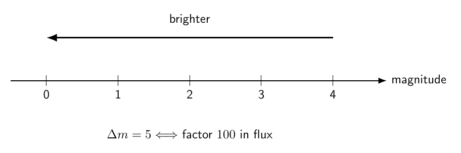
Figure 2. The astronomical magnitude scale is logarithmic and reversed: brighter sources have
smaller magnitudes. Five magnitudes correspond to a factor of one hundred in flux.
5 Example 1: flux ratio from magnitude difference
Suppose two stars differ by
Then
 | = 10−0.4(2.0) | (12)
|
| = 10−0.8 | (13)
|
| ≈ 0.1585. | (14) |
Thus
A two-magnitude difference is therefore much larger than a factor of two in flux.
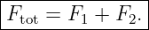
6 Combined light from an unresolved binary
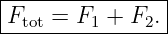
If both stars fall inside the same aperture, fluxes add linearly:
Magnitudes do not add.
Let the component magnitudes in the same band be m1 and m2.
Using an arbitrary common zero-point flux F0,
and
Therefore the combined magnitude is
when the same magnitude zero point is used for both stars.
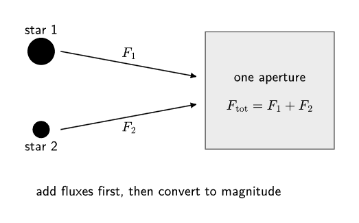
Figure 3. In an unresolved binary the detector records the sum of component fluxes. Magnitudes
must be converted to linear flux units before the component contributions are added.
7 Equal stars and the 0.7526 magnitude result
If two unresolved components have equal flux F,
The combined system is brighter by
| Δm | = −2.5 log 10(2) | (21)
|
| ≈−0.7526. | (22) |
Therefore
This is a useful binary star sanity check.
An unresolved equal-luminosity binary lies about 0.75 magnitude above the corresponding
single-star sequence if distance and extinction are the same.
8 Flux ratios and eclipse depth
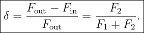
Suppose star 2 contributes flux F2 and is completely hidden while star 1 remains visible.
Out of eclipse,
During the total eclipse of star 2,
The fractional eclipse depth is
Thus a photometric eclipse can directly constrain a component flux ratio when the eclipse
geometry is sufficiently simple.
9 Color indices
A color index is a magnitude difference between two passbands.
For example,
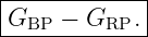
Gaia commonly provides
Color is related to the shape of the spectral energy distribution and therefore to effective
temperature, extinction, surface gravity, and composition.
For an unresolved binary, the system color is produced by the sum of the component fluxes in each
band.
It is not generally the arithmetic average of the component colors.
10 A binary can change color during eclipse
If two stars have different temperatures, their spectral energy distributions differ.
During an eclipse, the relative contribution of each star changes.
Therefore the observed color can change with orbital phase.
Multi-band eclipse photometry can therefore constrain
- surface-brightness ratio,
- temperature ratio,
- third Light,
- wavelength-dependent limb darkening.
This becomes important later in the eclipsing-binary sequence.
11 Extinction and reddening
Interstellar dust removes and redistributes light.
A simple passband extinction relation is
where m0 is the unextinguished magnitude and Aλ is the extinction in that band.
Because extinction depends on wavelength, dust also changes colors.
A common color excess is
Binary stars do not avoid extinction merely because the two components are at the same
distance.
The advantage is that both components usually experience nearly the same foreground extinction,
which can simplify differential comparisons.
12 Right ascension and declination
The standard equatorial coordinates are right ascension and declination.
Right ascension is analogous to longitude on the Celestial Sphere.
Declination is analogous to latitude.
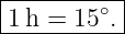
Right ascension is often expressed in hours, minutes, and seconds:
Thus
Declination is measured in degrees north or south of the Celestial Equator.
A catalog position is incomplete unless the coordinate frame and reference epoch are
understood.
13 Small angular offsets on the sky
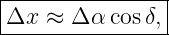
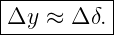
For two nearby sky positions with small separations,
and
The tangent-plane east-west offset is approximately
while the north-south offset is
The small-angle separation is
This is useful for resolved binary astrometry, but great-circle formulas should be used when
separations are not small.
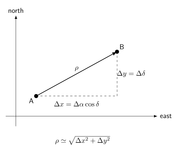
Figure 4. Small binary star separations can be described in a local tangent plane. The
right-ascension difference must be multiplied by cosδ when converting to an east-west angular
offset.
14 Position angle
For resolved binary stars, a relative position is often described by separation
and position angle
Position angle is conventionally measured from north through east on the sky.
With local offsets
toward east and
toward north,
The two-argument arctangent is important because it preserves the correct quadrant.
15 Time is a physical coordinate in binary star astronomy
For a binary star, the observation time is part of the measurement.
Orbital phase, eclipse timing, radial velocity, and astrometric position all depend on
time.
An observation should therefore be thought of as a pair:
Poor time bookkeeping can create a false phase shift even when the flux or velocity measurement
itself is perfect.
16 UTC, TT, TDB, and barycentric timing
Several time standards appear in astronomical work.
- UTC is the civil time scale used for timestamps and includes leap seconds.
- TT is a uniform terrestrial time scale used in ephemeris-related calculations.
- TDB is a relativistic time coordinate convenient for Solar-system barycentric dynamics.
- Barycentric timestamps account for the changing light-travel time between the
observatory and the Solar-system barycenter.
For precision binary star timing, simply recording a UTC date is often not sufficient.
17 Julian Date and Modified Julian Date
Julian Date is a continuous day count.
Modified Julian Date is defined by
The offset places the MJD day boundary at midnight rather than noon and reduces the numerical
size of the date.
The time standard must still be specified.
For example,
and
are not identical quantities.
18 Barycentric Julian Date
A common precision-timing quantity is Barycentric Julian Date.
In binary star photometry one often encounters
It combines a barycentric light-travel correction with a uniform relativistic time scale.
The exact transformation depends on
- observatory location,
- target coordinates,
- Solar-system ephemeris,
- original time standard.
Therefore the phrase “Julian Date” alone can be inadequate for high-precision eclipse
timing.
19 TESS time
TESS light-curve products commonly use a truncated barycentric time coordinate.
A frequently used convention is
The FITS header and data-product documentation should always be checked rather than assuming
an offset.

Figure 5. Precision binary star timing requires both a numerical date convention and a time
standard. Archive products may store barycentric times with mission-specific offsets.
20 Cadence and exposure time
An astronomical time series consists of finite exposures, not infinitely short samples.
Let
be the exposure time and
the cadence between reported samples.
If an eclipse ingress lasts only a few exposure times, finite integration can smear its
shape.
This matters because ingress and egress durations constrain stellar radii and inclination.
A forward model should ideally be integrated over the same exposure duration as the
data.
21 Uncertainty and signal-to-noise ratio
A measurement without an uncertainty has limited scientific meaning.
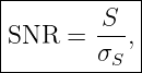
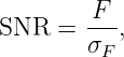
A simple signal-to-noise ratio is
where S is a measured signal and σS is its standard uncertainty.
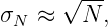
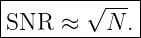
For ideal Poisson counting statistics with negligible background,
so
Real astronomical data also contain background noise, read noise, calibration uncertainty,
contamination, and astrophysical variability.
22 Magnitude uncertainty from flux uncertainty
For
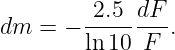
a first-order differential gives
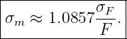
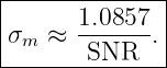
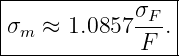
Therefore the approximate magnitude uncertainty is
Since
This approximation is best when the fractional flux uncertainty is small.
23 Why many catalogs prefer flux-space errors
A magnitude is a nonlinear logarithmic transformation of flux.
A symmetric Gaussian error in flux becomes asymmetric after transformation into magnitude.
For that reason, modern catalogs can report mean flux and flux error as the fundamental
measurement while providing a magnitude derived from that mean flux.
This is the approach used for Gaia mean broad-band photometry.
For rigorous uncertainty propagation, working in flux space is often preferable.
24 Spectra
A spectrum records flux as a function of wavelength or frequency.
A simplified one-dimensional spectrum is
A binary spectrum can contain lines from one star, both stars, circumstellar gas, or blended
combinations of all of these.
As orbital phase changes, photospheric lines can shift in wavelength because of the line-of-sight
velocity of each component.
This leads to the spectroscopic-binary method developed later in the series.
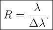
25 Spectral resolving power
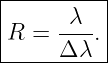
The resolving power of a spectrograph is
At wavelength
a spectrograph with
has characteristic resolution
| Δλ | =  | (63)
|
| = 0.025 nm. | (64) |
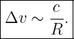
An equivalent velocity scale is approximately
This is a resolution scale, not automatically the final radial-velocity precision.
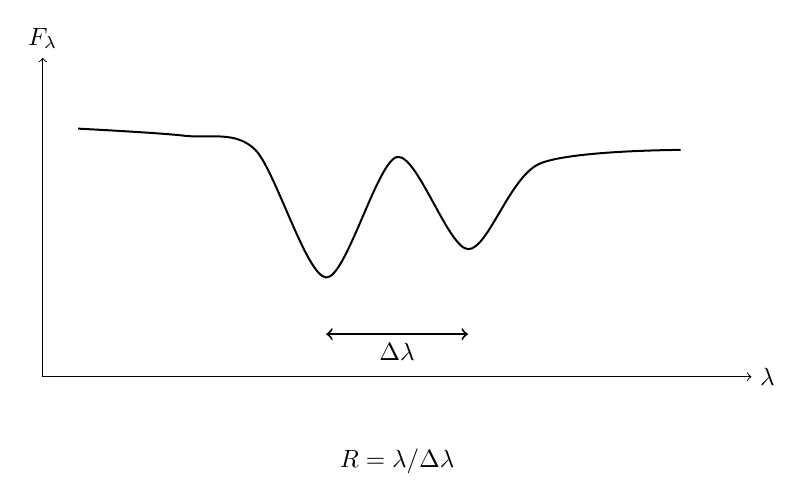
Figure 6. Spectral resolving power measures the ability to separate nearby wavelengths. Higher
resolving power reveals narrower and more clearly separated line structure.
26 Doppler shift preview
For nonrelativistic radial speed,
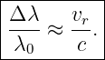
the wavelength shift is approximately
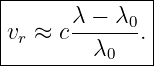
Thus
The sign convention must be stated.
A common convention assigns positive radial velocity to recession.
Full radial-velocity extraction is postponed until BIN07 and BIN20.
27 The FITS format
The Flexible Image Transport System, or FITS, is a standard astronomical data format.
A FITS file can contain multiple header-data units, usually abbreviated HDUs.
A typical file can include
- a primary HDU,
- one or more image HDUs,
- one or more binary-table HDUs.
Each HDU contains a header describing the data and, when applicable, a data block.
Important header metadata can include
- target identifier,
- coordinate information,
- time system,
- units,
- instrument,
- exposure time,
- processing level,
- quality or provenance keywords.
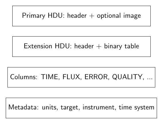
Figure 7. A FITS file can contain several header-data units. Scientific interpretation requires
reading the metadata as well as the numerical array or table.
28 Binary tables in time-series FITS files
A light-curve FITS product often stores one observation per row in a binary table.
Typical columns can include
- time,
- flux,
- flux uncertainty,
- background,
- centroid position,
- quality flags.
Mission-specific names must be read from the product documentation.
For TESS, commonly encountered columns include
and
The former is based on simple aperture photometry.
The latter applies corrections intended to reduce common instrumental systematics.
29 Quality flags are data
A quality flag is not decorative metadata.
It tells the user that a sample may have been affected by events such as
- spacecraft pointing changes,
- cosmic rays,
- momentum dumps,
- scattered light,
- detector anomalies.
A reproducible analysis must state how quality flags were handled.
Different scientific goals can justify different masks.
30 Gaia mean photometry
Gaia DR3 reports mean fluxes and flux uncertainties in its broad photometric bands, including G,
GBP , and GRP .
The catalog also provides corresponding mean magnitudes.
A useful observational lesson is that the magnitude values are derived from mean fluxes.
The archive documentation explicitly warns that a symmetric flux uncertainty does not transform
into a single symmetric magnitude uncertainty.
This is a concrete example of why one should understand the native measurement space.
31 TESS SAP and PDCSAP flux
TESS light-curve files available from MAST commonly contain both SAP and PDCSAP
flux.
SAP flux is the aperture-summed signal after the pipeline’s basic photometric extraction.
PDCSAP flux attempts to remove instrumental trends using cotrending information.
Neither column should be treated as automatically perfect.
For eclipsing binary work, detrending choices can influence eclipse depth, baseline shape, and
inferred parameters.
The rawer SAP series and the corrected PDCSAP series are therefore both scientifically
useful.
32 Blending and third light
A photometric aperture can contain flux from stars other than the two modeled binary
components.
Let the contaminating flux be
Then
The contaminating term is often called third light even when it comes from an unrelated
background star.
Third light dilutes eclipse depth.
A shallow observed eclipse can therefore be caused by
- a genuinely small blocked flux fraction,
- grazing geometry,
- a faint eclipsed star,
- contaminating third light,
- some combination of these effects.
33 Normalization
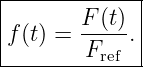
Time-series photometry is often normalized by a representative out-of-eclipse flux.
For example,
Then the out-of-eclipse baseline is near
A differential magnitude can be defined by
Normalization is a mathematical convenience.
It should not erase the distinction between calibrated absolute photometry and relative light-curve
shape.
34 From archive query to reproducible measurement
A defensible archive workflow should preserve:
- archive name,
- target identifier,
- query or cone-search region,
- retrieval date,
- data release,
- file identifier,
- units,
- quality-mask rule,
- software version,
- processing choices.
A result is not fully reproducible if only the final plot is saved.

Figure 8. A reproducible binary star data workflow preserves archive identity, query details,
metadata, quality filtering, processing choices, and derived products.
35 Live data and frozen data
The BIN series uses two complementary ideas.
A live query teaches how to interact with a professional archive.
A frozen extract preserves a small subset of the data so that the lesson still works if
- an archive interface changes,
- a catalog is updated,
- network access is unavailable,
- a source is reprocessed.
The frozen data are not meant to replace the live archive.
They provide a reproducible checkpoint.
36 Example 2: eclipse depth in flux and magnitudes
Suppose the normalized flux outside eclipse is
and at mid-eclipse is
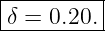
The fractional depth is
The differential magnitude at mid-eclipse is
| Δm | = −2.5 log 10(0.80) | (79)
|
| ≈ 0.242. | (80) |
Thus
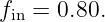
A 20% flux loss is not a 0.20 magnitude change because magnitudes are logarithmic.
37 Example 3: timing offset
Suppose a TESS measurement has
Using
the corresponding barycentric Julian Date is
The numerical offset must be restored before comparing to a literature ephemeris expressed in full
BJD.
38 Example 4: photon-limited uncertainty
If a detector records
photoelectrons and photon noise dominates,
Therefore
The approximate magnitude uncertainty is
| σm | ≈ | (88)
|
| ≈ 0.00109 mag. | (89) |
This is about one millimagnitude.
Real observations can have a larger uncertainty because photon noise is rarely the only noise
source.
39 A practical observational checklist
Before interpreting an archive measurement, ask:
- What quantity did the detector actually measure?
- What calibration produced the reported flux or magnitude?
- What passband is being used?
- Is the binary resolved or blended?
- What coordinate frame and epoch are attached to the position?
- What time standard and numerical offset are attached to the timestamp?
- What are the uncertainty and quality flags?
- Is the measurement raw, calibrated, or detrended?
- Is there contamination from neighboring sources?
- Can the exact archive query and processing steps be reproduced?
40 Common mistakes
- Adding magnitudes instead of fluxes.
- Comparing magnitudes from different passbands as though they measured the same
quantity.
- Forgetting that smaller astronomical magnitude means brighter flux.
- Treating an unresolved binary magnitude as the magnitude of one component.
- Averaging component colors instead of adding component fluxes band by band.
- Using right-ascension differences without the cos δ factor in a small tangent-plane
calculation.
- Omitting coordinate frame or reference epoch.
- Writing “JD” without checking the underlying time standard.
- Comparing BTJD directly with a full BJD ephemeris without restoring the mission
offset.
- Ignoring finite exposure time near sharp eclipse features.
- Assuming photon noise is the only uncertainty.
- Propagating a symmetric flux error into a symmetric magnitude error when the
fractional error is large.
- Treating resolving power R as identical to final radial-velocity precision.
- Reading a FITS data array without inspecting its header.
- Ignoring quality flags.
- Assuming PDCSAP is always scientifically preferable to SAP.
- Ignoring aperture contamination or third light.
- Saving a plot without recording the archive query, software, and data release.
41 Practice exercises
- A binary component is 3.0 magnitudes fainter than its companion in the same passband.
Find the flux ratio.
- Two unresolved stars have magnitudes 8.0 and 9.0 in the same band. Find the combined
magnitude.
- Show that two equal-flux unresolved stars are 0.7526 magnitude brighter than either
component alone.
- A total eclipse removes 30% of the out-of-eclipse flux. Find the corresponding
differential magnitude.
- A source has GBP = 10.4 and GRP = 9.7. Find GBP − GRP .
- Convert right ascension 6 h to degrees.
- Two resolved components differ by 0.80 arcsec in right ascension coordinate at
declination 60∘ and by 0.30 arcsec in declination. Find the approximate tangent-plane
separation.
- Derive the position-angle expression using east and north offsets.
- Convert MJD 60000 to JD.
- Convert BTJD 1400 to full BJD using the standard TESS offset adopted in this article.
- A light curve has normalized flux 0.92 at eclipse minimum. Find the differential
magnitude.
- If SNR = 250, estimate the small-error magnitude uncertainty.
- A spectrograph has R = 50000. Estimate the velocity resolution scale c∕R.
- A spectral line at 500.000 nm is observed at 500.050 nm. Estimate the nonrelativistic
radial velocity.
- Explain why the same TESS aperture can produce different eclipse depths if an
unrelated contaminating star is added to the aperture.
42 Summary
Flux and luminosity are connected by
Magnitudes encode flux ratios:
Unresolved binary fluxes add linearly:
Precision binary star astronomy requires explicit coordinates and time standards.
For TESS-like barycentric times,
For small relative flux error,
Spectral resolving power is
FITS data products combine numerical data with metadata that are necessary for physical
interpretation.
These observational tools provide the measurement foundation for BIN03, where the series turns
from measured positions and times to Newtonian two-body dynamics and Keplerian
orbits.
References
References
[1] B. W. Carroll and D. A. Ostlie, An Introduction to Modern Astrophysics, 2nd ed.,
Cambridge University Press, 2017.
[2] S. B. Howell, Handbook of CCD Astronomy, 2nd ed., Cambridge University Press,
2006.
[3] Gaia Collaboration, Gaia Data Release 3: Summary of the Content and Survey
Properties, Astronomy and Astrophysics, 674, A1, 2023.
[4] ESA and Gaia DPAC, Gaia Data Release 3 Documentation, Gaia Archive Data
Model, release 1.3, 2023.
[5] G. R. Ricker et al., Transiting Exoplanet Survey Satellite, Journal of Astronomical
Telescopes, Instruments, and Systems, 1, 014003, 2015.
[6] P. F. L. Maxted et al., The TESS Light Curve of AI Phoenicis, Monthly Notices of
the Royal Astronomical Society, 498, 332–343, 2020.
[7] D. C. Wells, E. W. Greisen, and R. H. Harten, FITS: A Flexible Image Transport
System, Astronomy and Astrophysics Supplement Series, 44, 363–370, 1981.
[8] Astropy Collaboration, The Astropy Project: Sustaining and Growing a
Community-Oriented Open-Source Project and the Latest Major Release, Astrophysical
Journal, 935, 167, 2022.