Drag Forces and Terminal Velocity

A body moving through a fluid usually experiences a resistive force called drag. Unlike Weight or an ideal spring force, drag depends on the body’s motion relative to the surrounding fluid. That dependence makes drag problems an important first step beyond constant-force dynamics.

The most important modeling principle is that drag opposes the relative velocity between the body and the fluid. If

vrel = vbody − vfluid,

(1)

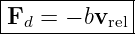
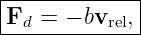
then a common linear model is

|------------| |Fd = − bvrel,| --------------

(2)

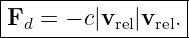
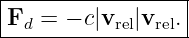
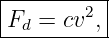
and a common quadratic model is

|-----------------| Fd = − c|vrel|vrel. | ------------------

(3)

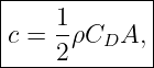
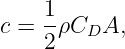
For aerodynamic drag, the quadratic coefficient is often written

|------------| | 1 | |c = -ρCDA, | -----2--------

(4)

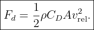
so that the drag magnitude becomes

|-----1----------| Fd = -ρCDAv2rel.| ------2-----------

(5)

This article develops both models, derives terminal velocity, solves the time-dependent falling problem for linear drag and for quadratic drag from rest, and shows how geometry, fluid density, and body mass affect the result.

1 Drag depends on relative motion

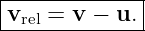
Suppose an object has velocity v in the laboratory frame while the surrounding fluid has local velocity u. The relative velocity seen by the fluid is

|------------| vrel = v − u.| --------------

(6)

The drag force points opposite this vector.

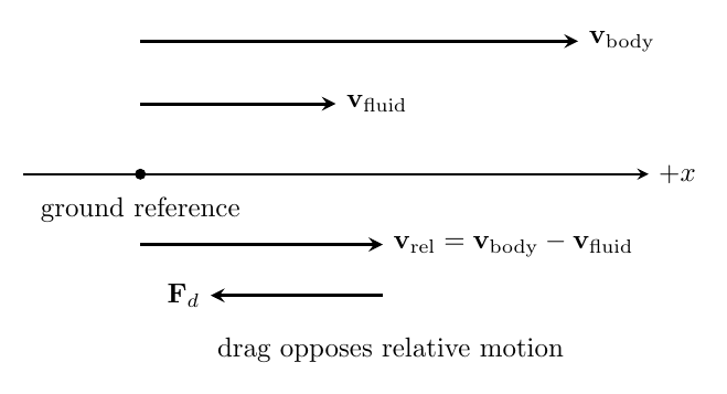
Figure 1. Drag is determined by the body’s velocity relative to the fluid, not necessarily by its velocity relative to the ground. A following wind can reduce the relative airspeed and therefore reduce aerodynamic drag.

This distinction matters whenever the fluid itself moves. For example, a cyclist moving east at 12 m∕s through air moving east at 5 m∕s has an air-relative speed of only 7 m∕s.

2 Linear and quadratic drag models

Two idealized drag laws appear frequently in mechanics.

For linear drag,

|--------| -Fd-=-bv,-

(7)

where b has SI units

[b] = N-s . m

(8)

For quadratic drag,

|----------| |Fd = cv2, | -----------

(9)

where

kg- [c] = m .

(10)

The two models have different speed dependence.

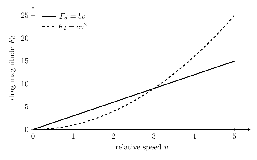
Figure 2. Linear drag grows in direct proportion to relative speed, while quadratic drag grows as the square of relative speed. The appropriate model depends on the flow regime and object geometry.

Linear drag is especially important for sufficiently slow motion in viscous flow. Quadratic drag is commonly useful for many macroscopic bodies moving through air or water at moderate to high Reynolds number.

3 A brief note on Reynolds number

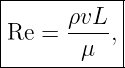
The dimensionless Reynolds number compares inertial effects in the fluid with viscous effects. A common form is

|----------| | ρvL- | Re = μ ,| ------------

(11)

where ρ is fluid density, v is a characteristic relative speed, L is a characteristic length, and μ is dynamic viscosity.

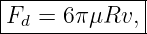
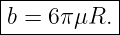
Very low Reynolds number flow around a small sphere can lead to Stokes drag,

|-------------| Fd = 6πμRv, | ---------------

(12)

which is linear in speed. In that case,

|----------| |b = 6πμR. | ------------

(13)

At larger Reynolds number, the drag law is generally more complicated, and a quadratic approximation is often more useful. The exact transition between regimes is a fluid-mechanics question; the present article uses the two models as controlled approximations.

4 Terminal velocity as a force-balance state

Consider a body falling vertically through still fluid. Take downward as positive. Its weight points downward while drag points upward.

If buoyancy is negligible, Newton’s second law is

mg − Fd = ma.

(14)

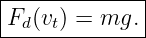
At terminal velocity, the speed is constant, so

a = 0.

(15)

Therefore the terminal-speed condition is

|------------| Fd (vt) = mg. | --------------

(16)

The body is still moving. Terminal velocity means zero acceleration, not zero velocity.

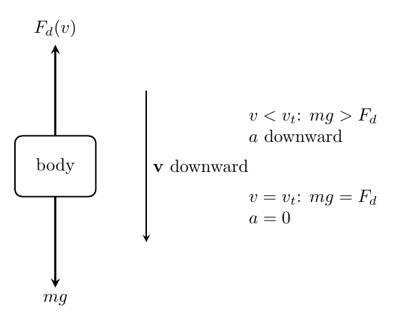
Figure 3. During downward fall, weight drives the motion and drag opposes it. At terminal velocity the forces balance, so the acceleration is zero even though the body continues moving.

5 Terminal speed with linear drag

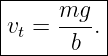
For linear drag,

Fd = bv.

(17)

At terminal speed,

mg = bvt.

(18)

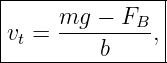
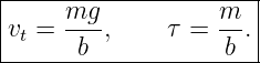
Hence

|----------| | mg-- | -vt-=--b-.-|

(19)

Thus the linear-drag terminal speed increases directly with mass and decreases inversely with the drag coefficient.

6 Transient fall with linear drag

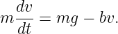
With downward positive, the equation of motion is

dv m ---= mg − bv. dt

(20)

Using

vt = mg-, b

(21)

we can write

( ) dv- v- dt = g 1 − v . t

(22)

Define the time constant

|--------| | m- | -τ-=--b-.|

(23)

Then the general solution is

|-------------------------| | −t∕τ | v(t)-=-vt +-(v0-−-vt)e--.--

(24)

For release from rest, v₀ = 0, so

|--------------------| v(t) = v (1 − e−t∕τ).| --------t-------------

(25)

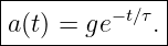
The acceleration is

|--------------| | −t∕τ | -a(t) =-ge----.

(26)

For release from rest at y = y₀, the downward displacement is

|------------------------------| | [ ( −t∕τ)] | -y −-y0 =-vt-t −-τ-1-−-e------.-

(27)

The speed approaches v_t exponentially rather than reaching it at a finite time in the ideal model.

7 Worked example 1: linear drag and approach to terminal speed

A 0.200 kg object falls from rest through a fluid with linear drag coefficient b = 0.800 N s∕m. Neglect buoyancy. Find the terminal speed, the time constant, the speed after 0.500 s, and the acceleration at that time.

The terminal speed is

mg-- (0.200)(9.81-) vt = b = 0.800 = 2.45 m ∕s.

(28)

The time constant is

τ = m- = 0.200--= 0.250 s. b 0.800

(29)

At t = 0.500 s,

( −t∕τ) −2 v = vt 1 − e = (2.45)(1 − e ) = 2.12 m∕s.

(30)

The acceleration is

a = ge− t∕τ = (9.81)e−2 = 1.33 m ∕s2.

(31)

Therefore

|---------------------------------------------------------------------------| | 2 | vt-=-2.45-m-∕s,--τ-=-0.250-s,--v(0.500)-=-2.12-m-∕s,--a(0.500)-=-1.33-m∕s-.--

(32)

8 Terminal speed with quadratic drag

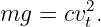
For quadratic drag,

2 Fd = cv .

(33)

At terminal speed,

2 mg = cvt.

(34)

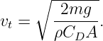
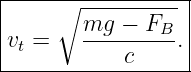
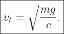
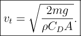
Therefore

|-----∘------| | mg | |vt = ----.| ---------c---

(35)

Using

c = 1ρCDA, 2

(36)

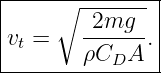
this becomes

|--------------| | ∘ -2mg---| |vt = ------.| --------ρCDA----

(37)

Several scaling laws follow immediately:

√ -- 1 1 1 vt ∝ m, vt ∝ √---, vt ∝ √--, vt ∝ √-----. A ρ CD

(38)

9 Transient fall with quadratic drag

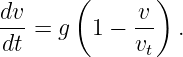
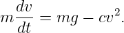
For downward motion through still fluid with v ≥ 0,

m dv-= mg − cv2. dt

(39)

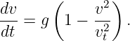
Since

2 mg-- vt = c ,

(40)

we obtain

dv ( v2) ---= g 1 − -2- . dt vt

(41)

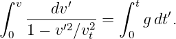
For release from rest, separation of variables gives

∫ v dv ′ ∫ t -----′2--2 = g dt′. 0 1 − v ∕vt 0

(42)

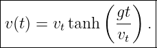
The result is

|-------------(---)--| | gt | v (t) = vttanh v- .| -----------------t----

(43)

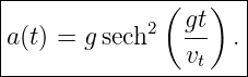
The acceleration is

|-------------(---)--| | 2 gt | a (t) = g sech -- .| ----------------vt----

(44)

For release from rest, the downward displacement is

|--------------[----(----)]--| | v2t- gt | |y − y0 = g ln cosh v .| -----------------------t-----

(45)

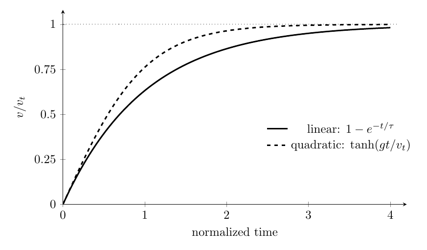
Figure 4. Linear and quadratic drag both cause a falling body released from rest to approach a finite terminal speed asymptotically. The shapes differ because the resisting force has different speed dependence.

10 Worked example 2: quadratic drag in air

A 0.0750 kg object falls through air of density 1.20 kg∕m³. Let C_D = 0.470 and A = 3.00 × 10⁻³ m². Assume quadratic drag and neglect buoyancy. Find the terminal speed and the speed after 2.00 s if released from rest.

The quadratic coefficient is

1- 1- −3 −4 c = 2ρCDA = 2(1.20)(0.470)(3.00 × 10 ) = 8.46 × 10 kg∕m.

(46)

Thus

∘ ---- ∘ --------------- v = mg--= (0.0750-)(9.81)-= 29.5 m ∕s. t c 8.46 × 10−4

(47)

After 2.00 s,

( ) ( ) gt (9.81)(2.00) v = vttanh -- = (29.5)tanh ------------ = 17.2 m ∕s. vt 29.5

(48)

Therefore

|----------------------------------------| |vt = 29.5 m ∕s, v(2.00 s) = 17.2 m ∕s.| -----------------------------------------

(49)

11 Changing area: why parachutes work

For quadratic drag,

∘ ------- v = -2mg--. t ρCDA

(50)

Increasing frontal area reduces terminal speed. Increasing the drag coefficient has the same qualitative effect.

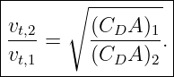
If the product C_DA changes from (C_DA)₁ to (C_DA)₂, then

|------------------| | ∘ | |vt,2-= (CDA--)1-.| |vt,1 (CDA )2 | -------------------

(51)

This square-root scaling is important. To reduce terminal speed by a factor of 3, the product C_DA must increase by a factor of 9.

12 Worked example 3: parachute deployment

A skydiver of mass 80.0 kg falls through air with density 1.20 kg∕m³. Before deployment, take C_D = 1.00 and A = 0.900 m². After deployment, take C_D = 1.40 and A = 18.0 m². Estimate the terminal speed before and after deployment.

Before deployment,

∘ ------- ∘ ------------------- v = -2mg--= ---2(80.0)(9.81)---= 38.1 m∕s. t,1 ρCDA (1.20)(1.00)(0.900 )

(52)

After deployment,

∘ ------------------ vt,2 = --2(80.0)(9.81)---= 7.20 m ∕s. (1.20)(1.40 )(18.0)

(53)

Thus

|------------------------------------| |vt,1 = 38.1 m ∕s, vt,2 = 7.20 m ∕s.| -------------------------------------

(54)

Immediately after deployment the skydiver may still be moving much faster than the new terminal speed, so the drag force can exceed the weight and produce a large upward acceleration.

13 Buoyancy and effective weight

For an object immersed in a fluid, the buoyant force can be important. If the object displaces fluid volume V , then

FB = ρfV g.

(55)

For downward motion, the force balance becomes

mg − FB − Fd = ma.

(56)

At terminal speed,

Fd (vt) = mg − FB.

(57)

Thus the effective downward driving force is the weight minus buoyancy.

For linear drag,

|----mg--−-F---| vt = --------B,| ---------b------

(58)

and for quadratic drag,

|----∘------------| | mg − F | vt = --------B. | -----------c-------

(59)

14 Worked example 4: Stokes drag with buoyancy

A small sphere of radius R = 2.00 mm and density 7800 kg∕m³ falls through an oil of density 900 kg∕m³ and dynamic viscosity 1.00 Pa s. Assume Stokes drag is valid. Find its terminal speed.

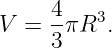
The sphere volume is

V = 4-πR3. 3

(60)

Its effective downward force is

(ρ − ρ )V g. s f

(61)

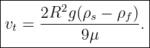
For Stokes drag,

Fd = 6πμRv.

(62)

At terminal speed,

4- 3 (ρs − ρf)3 πR g = 6πμRvt.

(63)

Solving,

|--------------------| | 2R2g (ρ − ρ ) | |vt = -------s----f-.| -----------9-μ-------

(64)

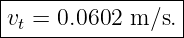
Substitution gives

−3 2 v = 2(2.00 ×-10--)-(9.81-)(7800-−--900)-= 6.02 × 10−2 m ∕s. t 9(1.00)

(65)

Therefore

|----------------| vt-=-0.0602-m-∕s.-

(66)

The corresponding Reynolds number is small, so the use of a linear Stokes model is self-consistent to first approximation.

15 What happens above or below terminal speed?

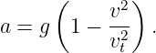
For downward fall with quadratic drag,

( v2) a = g 1 − -2- . vt

(67)

Therefore:

If 0 < v < v_t, then a > 0: the body speeds up downward.
If v = v_t, then a = 0: the speed remains constant.
If v > v_t, then a < 0: the acceleration points upward and the downward speed decreases.

This is why a parachute can slow a falling body. Deployment sharply lowers the new terminal speed while the actual speed initially remains large.

16 Common mistakes

Treating drag as opposite the ground-frame velocity instead of opposite the fluid-relative velocity.
Forgetting that terminal velocity means zero acceleration, not zero velocity.
Using F_d = cv² without separately tracking the direction of the force.
Mixing the linear and quadratic terminal-speed formulas.
Forgetting the square root in the quadratic result v_t = .
Assuming the drag coefficient C_D is a universal constant independent of shape and flow regime.
Ignoring buoyancy when the displaced-fluid weight is not negligible compared with the object’s weight.
Using Stokes drag at Reynolds numbers for which creeping-flow assumptions are not justified.

17 Practice problems

Use g = 9.81 m∕s² unless otherwise stated.

A CAR moves east at 30.0 m∕s while a wind blows east at 8.00 m∕s. Find the magnitude and direction of the car’s velocity relative to the air.
A 0.500 kg object falls through a fluid with linear drag coefficient b = 1.25 N s∕m. Neglect buoyancy. Find the terminal speed.
For the object in Problem 2, find the time constant and the speed after 1.00 s if released from rest.
A 2.00 kg object experiences quadratic drag F_d = cv² with c = 0.0800 kg∕m. Find its terminal speed.
A 0.120 kg object falls in air with ρ = 1.20 kg∕m³, C_D = 0.90, and A = 0.0100 m². Estimate its quadratic-drag terminal speed.
Under quadratic drag, an object’s mass is increased by a factor of 4 while ρ, C_D, and A remain unchanged. By what factor does its terminal speed change?
A parachute increases the product C_DA by a factor of 16. By what factor does the quadratic-drag terminal speed change?
A sphere of radius 1.50 mm moves slowly through a fluid of viscosity 0.800 Pa s. Find the linear drag coefficient b predicted by Stokes drag.
A submerged object has weight 12.0 N, buoyant force 3.00 N, and linear drag coefficient b = 4.50 N s∕m. Find its downward terminal speed.
A falling body obeys quadratic drag and has terminal speed 20.0 m∕s. At an instant when its downward speed is 12.0 m∕s, find the downward acceleration. At an instant when its downward speed is 25.0 m∕s, state the direction of its acceleration.

18 Answers

22.0 m∕s east relative to the air.
3.92 m∕s.
τ = 0.400 s; v = 3.60 m∕s downward.
15.7 m∕s.
14.8 m∕s.
A factor of 2 increase.
A factor of 1∕4; the new terminal speed is one-fourth the original.
b = 2.26 × 10⁻² N s∕m.
2.00 m∕s downward.
6.28 m∕s² downward at 12.0 m∕s; upward acceleration at 25.0 m∕s.

19 Summary

Drag is a velocity-dependent resistive force determined by motion relative to the fluid. The two ideal models emphasized here are

------------- |F = − bv | --d-------rel|

(68)

and

|-----------------| Fd-=--−-c|vrel|vrel.-|

(69)

For vertical fall with negligible buoyancy, terminal speed follows from the force balance F_d = mg.

For linear drag,

|----------------------| |vt = mg-, τ = m- .| -------b------------b--|

(70)

For quadratic drag,

|--------------| | ∘ -2mg---| |vt = ------.| --------ρCDA----

(71)

The terminal state is a dynamical balance: the body continues moving, but the net force and acceleration vanish.

References

[1] PhysicsLibrary, M02-01, Newton’s Laws of Motion.

[2] PhysicsLibrary, M02-03, Common Forces in Mechanics.

[3] OpenStax, University Physics, Volume 1, sections on drag force and terminal speed, CC BY 4.0.

[4] J. Moore et al., Mechanics Map, sections on drag forces and particle kinetics, CC BY-SA 4.0.

"Drag Forces and Terminal Velocity" is owned by bloftin.
(view preamble)