Wave Mechanics Examples: Traveling-Wave Solutions of the 1D Wave Equation
This companion article provides exercises for WM15, wave mechanics: Traveling-Wave Solutions of
the 1D wave equation. All exercises are stated first so they can be attempted without seeing the
answers. Complete worked solutions follow in Part II.
The central WM15 results are
for sufficiently smooth profile functions. The first-order direction tests are
and a sinusoidal solution must satisfy
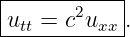
These results are standard consequences of the one-dimensional linear wave equation
[1, 2, 3, 4, 7].
How to use this problem set
For every proposed wave, separate three questions: what direction and speed are implied by the
argument; whether the function satisfies the PDE throughout the domain; and whether it also
satisfies the initial and boundary data of the particular physical problem.
Part I: Exercises
Exercise 1: Read direction and speed from the argument
For each function, state the propagation direction and speed magnitude:
| (a) | u = F(x − 6t), | (b) | u = G(x + 2.5t), | (4)
|
| (c) | u = H(3x − 12t), | (d) | u = Q(4x + 20t). | (5) |
For parts (c) and (d), first factor the argument into a constant times x ∓ ct.
Exercise 2: Verify the right-moving family
Let u(x,t) = F(x−ct) with F twice differentiable. Define ξ = x−ct. Derive ux, uxx, ut, and utt by
the chain rule and prove that utt = c2u
xx.
Exercise 3: Verify the left-moving family
Repeat Exercise 2 for u(x,t) = G(x + ct) using η = x + ct. Derive the first-order relation between
ut and ux that identifies leftward propagation.
Exercise 4: Infer speed from two snapshots

Figure. The same localized profile is observed at two times.
The center moves from x1 = 3.0 m at t1 = 0.20 s to x2 = 7.0 m at t2 = 0.70 s.
- Find Δt and Δx.
- Determine the propagation speed.
- Write a generic traveling-wave form using an arbitrary profile F.
- State the corresponding first-order relation between ut and ux.
Exercise 5: Construct solutions for a specified PDE
For
find the wave speed; write general right- and left-moving solutions; give one explicit smooth
right-moving Gaussian; and give one explicit left-moving sinusoid with k = 3 rad/m.
Exercise 6: Directly verify a Gaussian pulse
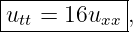
Test
against utt = 16uxx. Carry out the derivatives explicitly rather than appealing only to the general
theorem.
Exercise 7: Derive the sinusoidal solution condition
For
compute uxx and utt and derive the condition required by utt = c2u
xx. Then take c = 8 m/s and
k = 2.5 rad/m and determine ω and the ordinary frequency f.
Exercise 8: Read the ω-k solution test
For utt = 25uxx, the figure shows the allowed line and two candidate sinusoidal waves.
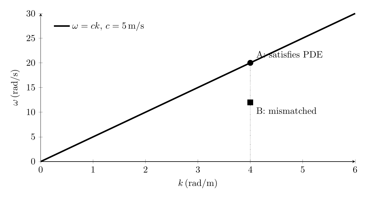
Figure. For c = 5 m/s, sinusoidal solutions must lie on ω = ck.
Candidate A has (k,ω) = (4, 20) and candidate B has (k,ω) = (4, 12) in SI-compatible
angular units. Decide which candidate satisfies the PDE, find the speed implied by
candidate B, and explain why agreement only at isolated zeros of the cosine would not be
sufficient.
Exercise 9: Direction from first-order derivatives
At one event a single shape-preserving traveling wave has
Determine the propagation direction and speed. Repeat if ut changes to +1.50 m/s while ux is
unchanged.
Exercise 10: Read characteristic lines

Figure. Constant values of x − ct and x + ct trace oppositely sloped feature trajectories in
the x-t plane.
Identify which line corresponds to x − ct = constant and which to x + ct = constant. Explain why
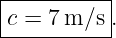
the second-order PDE supports both directions. If a right-moving line is x = 1.2t − 3, find its
speed.
Exercise 11: Superpose right- and left-moving solutions
Let u1 = F(x − ct) and u2 = G(x + ct), with both profiles twice differentiable. Use linearity to
prove that
also satisfies the wave equation. Explain why this does not yet determine F and G for a particular
initial-value problem.
Exercise 12: Propagate a prescribed initial shape
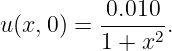
A right-moving pulse obeys utt = 100uxx and at t = 0 has
Find the speed, write u(x,t), write the profile at t = 0.30 s, and determine how far the center has
moved.
Exercise 13: Smoothness and the classical solution requirement
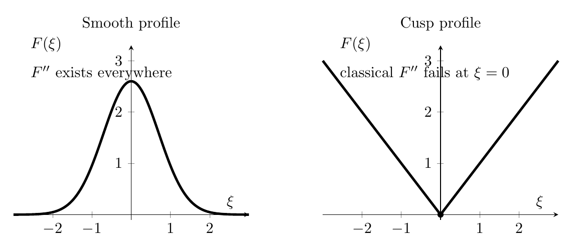
Figure. A smooth profile is compared with a cusp profile.
Compare u1 = e−(x−ct)2 with u
2 = |x − ct|. Which is a classical twice-differentiable solution
everywhere? Along what line does the cusp fail the WM15 smoothness assumption? What are u2,xx
and u2,tt away from that line?
Exercise 14: Synthesis - mechanics to traveling solution
An ideal string has
A right-moving sinusoid has wavelength λ = 1.50 m and amplitude A = 4.0 mm. At t = 0 it is at
maximum positive displacement at x = 0.
Find c, k, ω, and f; write a right-moving sinusoidal solution; verify μutt = Tuxx; and write the
corresponding left-moving sinusoid.
Part II: Complete Worked Solutions
Solution 1: Read direction and speed from the argument
Use F(x − ct) for rightward motion and G(x + ct) for leftward motion. Factoring the arguments
when necessary gives
| F(x − 6t) | : +x, c = 6 m/s, | (13)
|
| G(x + 2.5t) | : −x, c = 2.5 m/s, | (14)
|
H(3x − 12t) = H 3(x − 4t) 3(x − 4t) | : +x, c = 4 m/s, | (15)
|
Q(4x + 20t) = Q 4(x + 5t) 4(x + 5t) | : −x, c = 5 m/s. | (16) |
The prefactor multiplying the whole argument changes its spatial scale but not the translation
speed.
Solution 2: Verify the right-moving family
Let ξ = x − ct and u = F(ξ). Since ξx = 1 and ξt = −c, the chain rule gives
| ux | = F′(ξ), | uxx | = F′′(ξ), | (17)
|
| ut | = −cF′(ξ), | utt | = c2F′′(ξ). | (18) |
Therefore
The first time derivative also gives the directional relation ut = −cux.
Solution 3: Verify the left-moving family
Let η = x + ct and u = G(η). Here ηx = 1 and ηt = c, so
| ux | = G′(η), | uxx | = G′′(η), | (20)
|
| ut | = cG′(η), | utt | = c2G′′(η). | (21) |
Thus
The plus sign in the first-order relation distinguishes the left-moving family in this convention.
Solution 4: Infer speed from two snapshots
The measured differences are
Hence
Because the motion is toward increasing x, a generic form is
Solution 5: Construct solutions for a specified PDE
From utt = 49uxx,
Therefore the two traveling families are
One smooth Gaussian example is uR = e−(x−7t)2. For a left-moving sinusoid with k = 3 rad/m, the
required angular frequency is ω = ck = 21 rad/s, so one example is
Solution 6: Directly verify a Gaussian pulse
Set ξ = x − 4t and write u = 2e−ξ2. Differentiating the profile with respect to ξ gives
Because ξx = 1 and ξt = −4,
Hence
so the Gaussian is a classical right-moving solution.
Solution 7: Derive the sinusoidal solution condition
For u = A cos(kx − ωt + ϕ),
Substitution into the PDE requires ω2 = c2k2. For positive ω, k, and c,
With c = 8 m/s and k = 2.5 rad/m,
Solution 8: Read the ω-k solution test
The PDE utt = 25uxx requires c = 5 m/s and therefore ω = 5k.
Candidate A gives ω∕k = 20∕4 = 5 m/s, so it satisfies the PDE. Candidate B gives
ω∕k = 12∕4 = 3 m/s, so it does not.
At isolated zeros of the cosine, both sides of a mismatched PDE can vanish accidentally. A
solution must satisfy the equation throughout the relevant domain, not just at selected
points.
Solution 9: Direction from first-order derivatives
For a right-moving profile, ut = −cux. The given values have opposite signs, so
Thus the wave moves toward +x. If ut = +1.50 m/s while ux remains positive, then ut = +cux and
the wave moves toward −x with the same speed magnitude.
Solution 10: Read characteristic lines
A feature with x − ct = constant moves toward increasing x as t increases; a feature with
x + ct = constant moves toward decreasing x.
The second-order PDE contains c2, so the directional sign disappears after two time derivatives.
Both propagation directions therefore satisfy the same PDE.
For x = 1.2t − 3, the coefficient of t is the speed:
in the corresponding distance-per-time units.
Solution 11: Superpose right- and left-moving solutions
Each component satisfies the PDE:
For u = u1 + u2, linearity gives
| utt | = (u1)tt + (u2)tt | (39)
|
| = c2 (u
1)xx + (u2)xx (u
1)xx + (u2)xx![]](https://images.physicslibrary.org/cache/objects/1178/make4ht/WaveMechanicsExamplesTravelingWaveSolutionsOfThe1DWaveEquation33x.png) | (40)
|
| = c2u
xx. | (41) |
Therefore
is also a solution. The PDE alone does not determine the specific functions F and G; initial and
boundary data are needed to select them.
Solution 12: Propagate a prescribed initial shape
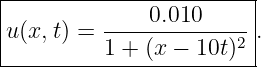
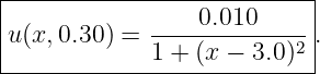
The PDE gives c =  = 10 m/s. The initial profile is F(x) = 0.010∕(1 + x2). Since the pulse is
known to move entirely toward +x,
= 10 m/s. The initial profile is F(x) = 0.010∕(1 + x2). Since the pulse is
known to move entirely toward +x,
At t = 0.30 s,
The center has moved ct = (10)(0.30) =
3.0 m .
Solution 13: Smoothness and the classical solution requirement
The Gaussian e−(x−ct)2 is smooth and has ordinary second derivatives everywhere. The cusp |x−ct|
fails to be differentiable in the ordinary sense along
Away from that line, the absolute-value profile is locally linear, so
At the cusp itself the classical second derivatives are not defined. Thus WM15’s statement about
arbitrary traveling profiles must be read as “arbitrary sufficiently smooth traveling profiles.”
More advanced PDE theory can treat nonsmooth profiles with generalized notions of
solution.
Solution 14: Synthesis - mechanics to traveling solution
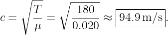
For an ideal string,
With λ = 1.50 m,
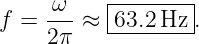
Hence
The phase condition u(0, 0) = +A is satisfied by zero phase constant, so the right-moving wave
is
For a sinusoid, uxx = −k2u and u
tt = −ω2u. Since ω2 = (T∕μ)k2,
Therefore the function satisfies the mechanical string equation. The corresponding left-moving
wave is
Common mistakes
- Reading H(3x − 12t) as a 12 m/s wave instead of first factoring the argument.
- Losing the minus sign in the first time derivative of F(x − ct).
- Carrying that minus sign into the second time derivative, where two factors of −c
produce +c2.
- testing a sinusoidal candidate at only one point instead of throughout the domain.
- Assuming the second-order wave equation by itself chooses a propagation direction.
- Treating a cusp exactly like a smooth classical solution.
- Forgetting that satisfying the PDE does not automatically satisfy a particular
problem’s initial or boundary conditions.
What WM15E1 reinforces
The main verification result is
for sufficiently smooth profiles. Direction is retained by the first-order relations, while the
second-order wave equation supports both directions. For sinusoidal waves the same requirement
becomes ω = ck.
The next stage can therefore ask the stronger question: given initial data, how are the two
traveling profiles F and G determined?
References
[1] A. P. French, Vibrations and Waves, M.I.T. Introductory Physics Series, W. W.
Norton & Company, 1971.
[2] Frank S. Crawford, Jr., Waves, Berkeley Physics Course, Volume 3, McGraw-Hill,
1968.
[3] William Moebs, Samuel J. Ling, and Jeff Sanny, University Physics, Volume 1,
OpenStax, 2016, Section 16.2, “Mathematics of Waves.”
[4] Richard P. Feynman, Robert B. Leighton, and Matthew Sands, The Feynman Lectures
on Physics, Volume I, Chapter 47, “Sound. The wave equation,” especially Section 47–4,
“Solutions of the wave equation.”
[5] Richard P. Feynman, Robert B. Leighton, and Matthew Sands, The Feynman Lectures
on Physics, Volume I, Chapter 48, “Beats,” including sinusoidal traveling waves and the
relation ω2 = k2c2.
[6] Richard P. Feynman, Robert B. Leighton, and Matthew Sands, The Feynman
Lectures on Physics, Volume I, Chapter 49, “Modes,” including the two-direction form
F(x − ct) + G(x + ct).
[7] Massachusetts Institute of Technology, 8.03SC Physics III: Vibrations and Waves,
Lecture 10, “Traveling Waves,” Fall 2016, MIT OpenCourseWare.

![[parent]](https://images.physicslibrary.org/images/uparrow.png)