Wave Mechanics: Oscillation at One Point
Before studying a wave that varies in both space and time, it is useful to understand the simpler
idea of oscillation at a single point. This article introduces a one-dimensional time-dependent
displacement u(t) and develops the ideas of equilibrium, displacement, amplitude, cycle,
period, and frequency. These quantities form the temporal foundation for later wave
mechanics.
Spatial periodicity, wavelength, Wavenumber, angular frequency, phase, and traveling-wave
equations are intentionally deferred to later lessons.
1 The simplest possible wave-mechanics starting point
Wave mechanics will eventually study fields such as
which can vary from place to place and from one instant to another. WM01 temporarily removes
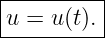
the spatial coordinate. We study only
This is not yet a traveling wave. It is one quantity changing with time at one location or for one
mechanical degree of freedom.
A mass attached to a spring is a useful mental model. The mass can move to either side of an
equilibrium position. Its displacement from equilibrium is described by the single number
u(t).
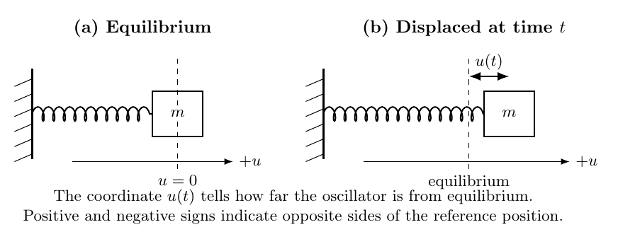
Figure. A one-dimensional oscillator. The reference position is called equilibrium and is
assigned u = 0. At any time t, the signed displacement u(t) tells how far the mass is from
equilibrium and on which side it lies.
The important abstraction is not the spring itself. Many systems can be described by a single
time-dependent variable: a pendulum angle, the vertical displacement of a floating object, the
voltage across an oscillating circuit element, or the pressure measured by a microphone at one fixed
location. The physical meaning changes, but the idea of a quantity varying with time remains the
same.
2 Equilibrium and displacement
An oscillator needs a reference position. We call this the equilibrium position. In this series the
displacement coordinate is normally chosen so that
at equilibrium.
The sign of u identifies which side of equilibrium the system occupies. For example,
| u(t) | > 0 | | means displacement in the chosen positive direction, | (4)
|
| u(t) | = 0 | | means the oscillator is at equilibrium, | (5)
|
| u(t) | < 0 | | means displacement in the opposite direction. | (6) |
The choice of positive direction is arbitrary, but it must be used consistently. Reversing the axis
changes the sign of u but does not change the physical motion.
2.1 Displacement is not distance traveled
Suppose the mass begins at u = 0, moves to u = +2 cm, then returns to u = 0. Its final
displacement is zero, but it has traveled a total distance of
Displacement describes location relative to equilibrium. Distance traveled describes the length of
the path taken during the motion. These are different quantities.
3 Amplitude
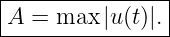
For an oscillation centered on equilibrium, the amplitude A is the largest magnitude of the
displacement:
Amplitude is therefore nonnegative:
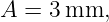
If the motion reaches +3 mm on one side and −3 mm on the other, then
not 6 mm. The full distance from one extreme to the other is 2A.
Amplitude answers the question
How large is the oscillation relative to equilibrium?
It does not tell us how quickly the oscillator moves or how many times per second the motion
repeats.
4 A time history
A graph of u versus t is called a time history. The horizontal axis represents time. The vertical axis
represents the value of the oscillating quantity.
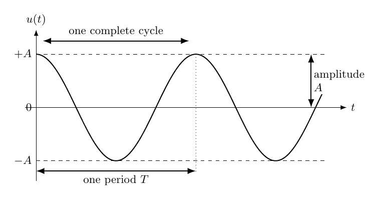
Figure. A schematic periodic time history. The amplitude A measures the maximum
displacement from equilibrium. The period T measures the time required for one complete
repetition. The precise sinusoidal formula for a smooth oscillation is introduced in WM02.
A time-history graph should not be confused with a picture of the physical path in space. In the
figure above, the curve does not mean that the oscillator travels along a wavy road. The curve
records the value of u(t) as time passes.
This distinction becomes even more important later, when a wave is described by a function of
both position and time.
5 Cycles and periodic motion
An oscillation is periodic when its motion repeats after a fixed amount of time.
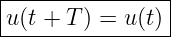
Mathematically, a function u(t) is periodic if there exists a positive number T such
that
for every time t for which the motion is defined.
A complete repetition of the motion is called a cycle. The time required for one cycle is called the
period.
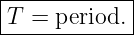
For a basic periodic oscillator, we use the symbol
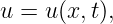
The SI unit of period is the second:
5.1 The smallest positive repeat time
If a motion repeats after T, it also repeats after 2T, 3T, and so on. When we speak of the
period, we normally mean the smallest positive time for which the complete pattern
repeats.
For example, if
for the complete repeating motion, then the period is
The motion also repeats after 0.50 s and 0.75 s, but these are multiples of the fundamental period
rather than new fundamental periods.
6 Returning to the same displacement is not necessarily one cycle
During one oscillation the system can pass through the same displacement more than
once.
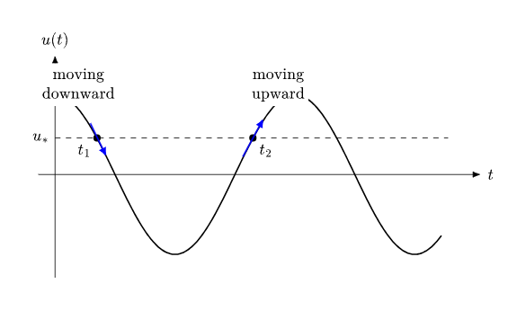
Figure. Two instants can have the same displacement u∗ while the oscillator moves in
opposite directions. Equal displacement does not by itself mean that the complete
mechanical state has repeated.
At the two marked times in the figure above,
but one crossing occurs while u is decreasing and the other while u is increasing.
For mechanical motion, a complete state includes more than position alone. velocity also matters.
When the full periodic motion repeats after one period, both the displacement and its
direction/rate of change repeat. This observation will later help motivate the concept of
phase.
7 Frequency
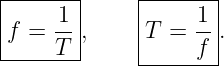
The period tells us how long one cycle takes. Frequency tells us how many cycles occur per unit
time.
If one cycle takes T seconds, then the number of cycles completed in one second is
The SI unit of frequency is the hertz:
Thus period and frequency contain the same timing information in reciprocal forms:
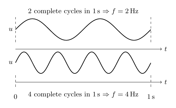
Figure. Frequency counts complete cycles per second. In the same one-second interval, the
lower-frequency motion completes fewer cycles and the higher-frequency motion completes
more.
7.1 Example: period to frequency
Suppose an oscillator completes one cycle every
Then
So the oscillator completes four cycles each second.
7.2 Example: frequency to period
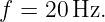
Suppose an oscillator has frequency
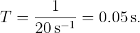
Then
Each cycle lasts 0.05 s.
8 Reading oscillation information from a graph
Given a time-history graph, use the following procedure.
- Identify the equilibrium value, normally u = 0.
- Measure the largest magnitude of the displacement to obtain the amplitude A.
- Choose a recognizable point in the cycle, such as a maximum.
- Find the next occurrence of the same point with the same direction of motion.
- Measure the time separation; this is the period T.
- Compute the frequency from f = 1∕T.
The phrase “same point with the same direction of motion” prevents the common mistake
illustrated earlier.
9 Units and dimensional checks
The basic quantities introduced in WM01 are summarized below.
| Symbol | Quantity | Typical SI unit | dimension |
|
|
|
|
| u(t) | displacement or oscillating variable | m for displacement | depends on variable |
| A | amplitude | same unit as u | same as u |
| T | period | s | time |
| f | frequency | Hz = s−1 | inverse time |
The relation
is dimensionally consistent because the reciprocal of seconds is inverse seconds. This kind of unit
check will become increasingly useful as more wave quantities are introduced.
10 What WM01 is deliberately not doing yet
Several familiar wave and oscillation quantities are intentionally absent from this lesson.
- No sinusoidal equation such as A cos(ωt + ϕ) is required yet.
- No angular frequency ω is required yet.
- No phase ϕ is required yet.
- No spatial coordinate x is being used.
- No wavelength λ or wavenumber k exists in this one-point description.
- No wave speed is being discussed because nothing is propagating through space yet.
This separation is intentional. Period and frequency are temporal concepts. Wavelength and
wavenumber will later be introduced as spatial concepts. Only after both sides are understood
separately will they be combined into a traveling wave.
11 Common misconceptions
11.1 Amplitude is not peak-to-peak motion
If the oscillator reaches +A and −A, its peak-to-peak range is
The amplitude remains A.
11.2 Frequency is not speed
A high frequency means many cycles occur per second. It does not by itself specify how
quickly a wave travels through space. Propagation speed is a different concept introduced
later.
11.3 Period is not wavelength
Period T measures a time interval. Wavelength λ measures a spatial interval. They have different
physical dimensions and should not be interchanged.
11.4 Crossing equilibrium is not the same as completing a cycle
An oscillator commonly crosses equilibrium twice during one complete cycle. Counting
equilibrium crossings without accounting for direction can therefore produce a factor-of-two
error.
12 A preview of the next step
WM01 has described periodic motion without specifying a particular mathematical shape.
In WM02 we will study the most important smooth periodic motion in physics: the
sinusoid.
The generic time-dependent variable
will become a specific function involving amplitude, a temporal rate of cycling, and an initial
position within the cycle. That will introduce angular frequency and phase while preserving the
period and frequency concepts developed here.
Summary
The essential results of WM01 are:
- An oscillation at one point is described by a time-dependent quantity u(t).
- Equilibrium is the reference position, normally chosen as u = 0.
- Displacement is signed; distance traveled is not the same thing as displacement.
- The amplitude A measures the maximum magnitude of the oscillation about
equilibrium.
- A periodic motion repeats after a period T:
- Frequency is the number of cycles per second and is the reciprocal of period:
- Returning to the same displacement does not necessarily mean a complete cycle has
occurred; direction of motion matters.
- No spatial wave quantities are needed yet. WM02 next introduces sinusoidal oscillation,
angular frequency, and phase.
Further reading
For complementary treatments of introductory oscillations, see A. P. French, vibrations and
Waves; Frank S. Crawford, Waves; and standard introductory university physics texts covering
oscillatory motion. The later articles in this series will develop the mathematical structure needed
for traveling waves, energy transport, boundary phenomena, Fourier methods, Helmholtz problems,
and quantum wave mechanics.




![[T] = s.](https://images.physicslibrary.org/cache/objects/1148/make4ht/OscillationAtOnePoint9x.png)