|
|
|
|||||||
when
Here
The central idea is simple:
For random orbital orientations, the fraction of allowed viewing directions turns out to be proportional to the fractional size
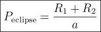
Under the ideal assumptions of a circular orbit, spherical stars, and random orientations, the result is actually stronger than an order-of-magnitude estimate:
provided
The approximate symbol in the introductory BIN01 discussion is useful because real binary stars can have eccentric orbits, distorted stars, detection thresholds, third Light, and incomplete observational coverage.
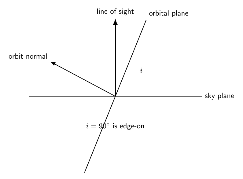
1 Orbital inclinationDefine orbital inclination i so that
A face-on binary shows the orbit nearly in its own plane on the sky and cannot produce ordinary stellar eclipses. An edge-on binary has one star pass directly in front of the other at conjunction. The eclipse question is therefore a question about how close i must be to
Figure 1. Inclination measures the tilt of the orbital plane relative to the sky. Eclipses require a viewing geometry close to edge-on.
2 Circular orbit geometry at conjunctionConsider a circular relative orbit of radius a. At conjunction, the relative separation vector is directed as nearly as possible along the observer’s line of sight. If the orbit is exactly edge-on,
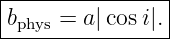
and the sky-plane separation of the stellar centers at conjunction is zero. If the orbit is tilted away from edge-on, the projected separation at conjunction is
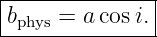
The symbol bphys here is a physical sky-plane offset, not a dimensionless impact parameter. For inclinations between
we can write simply
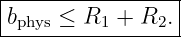
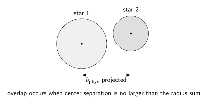
3 The eclipse criterionThe projected stellar disks overlap if the projected center-to-center separation is smaller than the sum of their radii:
Insert Equation (4):
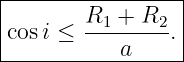
Divide by a:
Thus an eclipse occurs only for inclinations sufficiently close to edge-on.
Figure 2. At conjunction the stellar disks overlap when their projected center-to-center separation is no larger than the sum of the stellar radii.
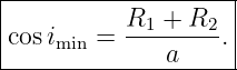
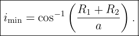
4 Minimum inclination for an eclipseDefine the limiting inclination imin by equality in Equation (6):
Therefore
An eclipse occurs when
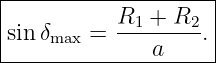
It is often useful to describe the same geometry by the small angular departure from exactly edge-on:
At the eclipse boundary,
Since
we have
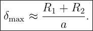
If
then δmax is small and
with δmax in radians. Thus
This is the first intuitive reason the eclipse probability should scale as stellar size divided by orbital size.
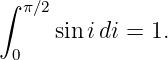
5 Random orbital orientationsThe missing step is probability. A population of randomly oriented orbital planes does not have a uniform distribution in inclination i. The orbital angular-momentum direction is isotropic on a sphere. The solid-angle element is
After folding the physically equivalent orientations i and 180∘− i, it is sufficient to consider
The normalized inclination probability density is
The normalization follows because
Equivalently,
This is the shortest route to the geometric eclipse probability.
6 Integrate over the eclipsing inclinationsThe probability of an eclipse is the probability that
Therefore
Using Equation (7),
This is the desired result. Notice that no small-angle approximation was required in the final probability integral. For the ideal circular geometry, Equation (13) follows exactly from isotropic orientation statistics.
7 The same result from uniform
|
 | (24) |
For random orientations,
 | (25) |
is uniform on the interval
 | (26) |
The eclipse condition is
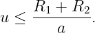 | (27) |
The probability is simply the length of the allowed interval divided by the length of the full interval:
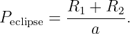 | (28) |
This is often the most efficient derivation used in transit and eclipsing-binary calculations.
There is also a useful geometric interpretation on the sphere of possible orbital-pole directions.
Eclipses occur when the orbit Normal lies in a narrow band around orientations corresponding to an edge-on orbit.
The half-width of that band is δmax.
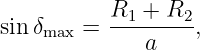
The fractional area of the band is
| (14) |
From Equation (9),
 | (29) |
so the same result follows.
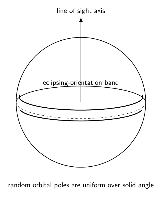
Figure 3. Random orbital poles are uniformly distributed over solid angle. Eclipsing systems occupy a narrow orientation band around edge-on viewing.
For the ideal circular model,
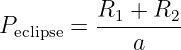 | (30) |
is a clean geometric result.
Real observations introduce additional effects:
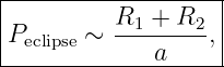
Thus it is useful in an introductory survey article to write
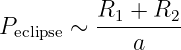 | (31) |
as an order-of-magnitude selection rule.
The present derivation shows the ideal geometric foundation beneath that estimate.
Equation (5) describes any overlap of the two projected stellar disks.
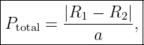
For a total eclipse of the smaller stellar disk, the projected center separation must satisfy
| (15) |
For a circular orbit with random orientation, the corresponding geometric probability is
| (16) |
provided the smaller star can be completely hidden by the larger disk.
The probability of a grazing-or-partial eclipse is therefore associated with the orientation interval between
 | (32) |
and
 | (33) |
For equal-radius stars,
 | (34) |
so a geometrically complete disappearance of one equal-sized disk occurs only for perfect projected alignment.
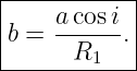
It is common to normalize the projected separation by a stellar radius.
For example, relative to star 1 define
| (17) |
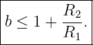
Then the any-overlap condition becomes
| (18) |
This form is closely related to the impact-parameter notation used in transit and eclipsing-binary light-curve modeling.
Consider two stars with approximately one solar radius each:
 | (35) |
Using
 | (36) |
we have
 | (37) |
Let the circular orbital separation be
 | (38) |
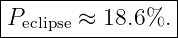
Then
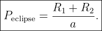
| Peclipse | =  | (39) |
| = 0.186. | (40) |
Therefore
| (19) |
The limiting inclination is
| imin | = cos −1(0.186) | (41) |
| ≈ 79.3∘. | (42) |
Thus this binary eclipses if it is viewed within about
 | (43) |
of exactly edge-on.
Keep the same two solar-radius stars but increase the orbital separation to
 | (44) |
Then
 | (45) |
Therefore
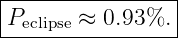 | (46) |
At
 | (47) |
the probability falls to approximately
 | (48) |
This is a strong geometric selection effect favoring close eclipsing binaries.
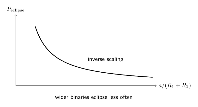
Figure 4. For fixed stellar radii, geometric eclipse probability decreases inversely with orbital separation.
Kepler’s third law gives
 | (49) |
Therefore
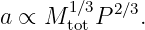 | (50) |
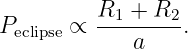
Insert this scaling into
 | (51) |
Then
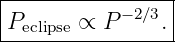
| (20) |
For broadly similar stellar masses and radii,
| (21) |
Short-period binaries are therefore much more likely to be found as eclipsing systems even before observational cadence and signal-to-noise effects are considered.
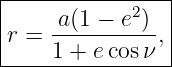
For an eccentric orbit, the star-to-star separation is not constant.
The radial separation is
| (22) |
where
The eclipse probability therefore depends on the separation at conjunction rather than simply on a.
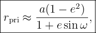
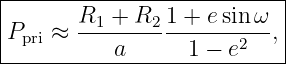
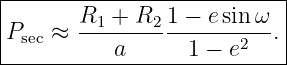
For nearly edge-on geometry, a common conjunction approximation gives
| (23) |
for one conjunction and
| (24) |
for the opposite conjunction, with the labeling depending on the adopted argument-of-periastron convention.
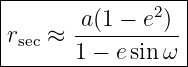
Replacing a by the conjunction separation gives
| (25) |
and
| (26) |
These formulas show that an eccentric binary is more likely to eclipse at a conjunction occurring near the smaller orbital separation.
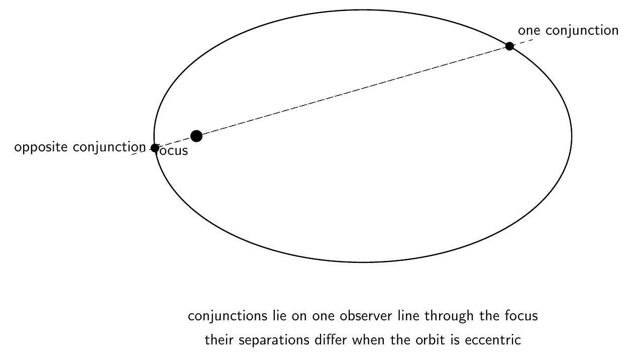
Figure 5. In an eccentric orbit the separation at conjunction depends on orbital orientation, so the geometric eclipse probability is no longer determined by the semimajor axis alone.
For a circular orbit, the separation is the same at both conjunctions.
If the geometry permits one stellar disk to overlap the other at one conjunction, the corresponding opposite conjunction also has an overlap geometry.
However, the two events need not have equal photometric detectability.
The primary and secondary eclipse depths depend on
A geometrically allowed secondary eclipse can therefore be too shallow to identify observationally.
For eccentric binaries, the two conjunctions occur at different separations, so their geometric eclipse conditions can differ.
Equation (13) answers only a geometric question:
 | (52) |
A survey detection probability contains additional factors.
Schematically,
| (27) |
This distinction becomes essential when inferring the intrinsic binary population from an eclipsing-binary catalog.
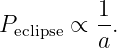
Suppose two populations contain the same intrinsic number of binaries but one population has systematically smaller orbital separations.
Even if the orbital orientations are equally random, the close population will contribute more eclipsing systems because
 | (53) |
An observed eclipsing-binary sample is therefore not a random sample of all binaries.
It is geometrically weighted toward
Correcting for this selection function is a major theme in modern population studies.
For a circular binary, the projected center separation at conjunction is
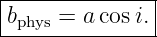 | (54) |
Any eclipse requires
 | (55) |
Thus
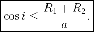 | (56) |
Random orbital orientations imply that cos i is uniformly distributed.
Therefore the fraction of orientations satisfying the eclipse condition is
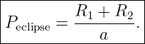 | (57) |
For
 | (58) |
the angular window around edge-on viewing is approximately
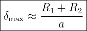 | (59) |
in radians.
The formula is therefore both a direct geometric probability and an intuitive statement that an eclipsing system must lie within a narrow orientation band whose angular width is set by stellar size divided by orbital size.
[1] B. W. Carroll and D. A. Ostlie, An Introduction to Modern Astrophysics, 2nd ed., Cambridge University Press, 2017.
[2] R. W. Hilditch, An Introduction to Close Binary Stars, Cambridge University Press, 2001.
[3] J. N. Winn, Exoplanet Transits and Occultations, in Exoplanets, edited by S. Seager, University of Arizona Press, 2010.
[4] D. Prialnik, An Introduction to the Theory of Stellar Structure and Evolution, 2nd ed., Cambridge University Press, 2009.
| Other names: | BIN01D4 |
| Also defines: | eclipse inclination criterion, random orbital orientation, grazing eclipse, total eclipse probability |
| Keywords: | binary stars, eclipsing binaries, eclipse probability, inclination, random orientation, geometric selection effect, impact parameter, stellar radii, orbital separation, eccentric orbit |
| Physics Classification: | 97.80.-d (Binary and multiple stars) |
None.
No messages.
![[parent]](https://images.physicslibrary.org/images/uparrow.png)




















![[− cosi]](https://images.physicslibrary.org/cache/objects/1417/make4ht/GeometricEclipseProbability31x.png)