example of Wave Mechanics: Wave Intensity and Flux

Wave Mechanics Examples: Wave Intensity and Flux

This companion article provides exercises for WM21, wave mechanics: Wave Intensity and flux. All exercises are stated first. Complete worked solutions follow in Part II.

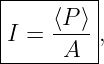
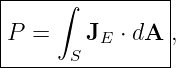
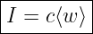
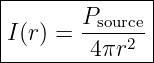
The central WM21 relations are

|--------| | ⟨P⟩-| I = A , ----------

(1)

|-----∫---------| |P = JE ⋅ dA , -------S---------

(2)

|--------| I-=-c⟨w-⟩-

(3)

for a progressive nondispersive wave, and

|--------------| |I(r) = Psource | ---------4πr2--|

(4)

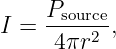
for an ideal isotropic spherical source [3, 4, 1, 2].

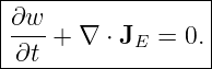
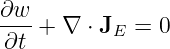
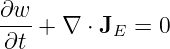
The corresponding local conservation law is

|------------------| |∂w | |-∂t + ∇ ⋅ JE = 0.| -------------------

(5)

How to use this problem set

Attempt all problems in Part I before reading Part II. In each calculation, first identify whether the quantity requested is total power in watts, intensity in watts per square meter, energy density in joules per cubic meter, or a directional flux. Many mistakes in this topic come from mixing these quantities.

Part I: Exercises

Exercise 1: Convert power to intensity

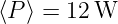
A uniform wave carries average power

⟨P ⟩ = 12 W

(6)

through a perpendicular area

2 A = 0.080 m .

(7)

Find the intensity and state its SI units.

Exercise 2: Same power, different area

The figure below shows the same total average power passing through two different perpendicular areas.

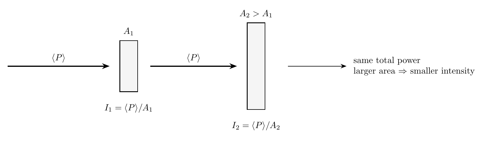
Figure. The same transported power spread over a larger area produces a smaller intensity.

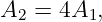
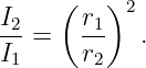
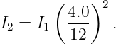
Suppose

A = 4A . 2 1

(8)

Find I₂∕I₁.
If I₁ = 80 W∕m², find I₂.
Does the decrease in intensity necessarily mean energy was dissipated? Explain.

Exercise 3: Flux through a tilted surface

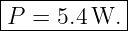
A uniform energy-flux vector has magnitude

2 JE = 18W ∕m .

(9)

It crosses a flat surface of area

A = 0.60 m2

(10)

at an angle

α = 60 ∘

(11)

with the surface normal.

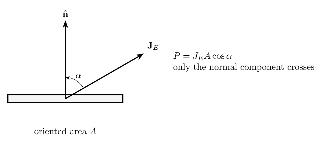
Figure. Only the component of the energy flux normal to the surface contributes to the signed power crossing it.

Find the power crossing the surface.

Exercise 4: Intensity from volume energy density

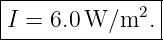
A progressive nondispersive wave has average volume energy density

⟨w ⟩ = 0.024 J∕m3

(12)

and propagation speed

c = 250 m/s.

(13)

Find the intensity.
Find the average power through a perpendicular area of 0.30 m².

Exercise 5: Spherical spreading ratio

An ideal isotropic source produces intensity

I1 = 0.36W ∕m2

(14)

at radius

r1 = 2.0m.

(15)

Find the intensity at

r = 5.0 m 2

(16)

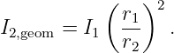
assuming no absorption.

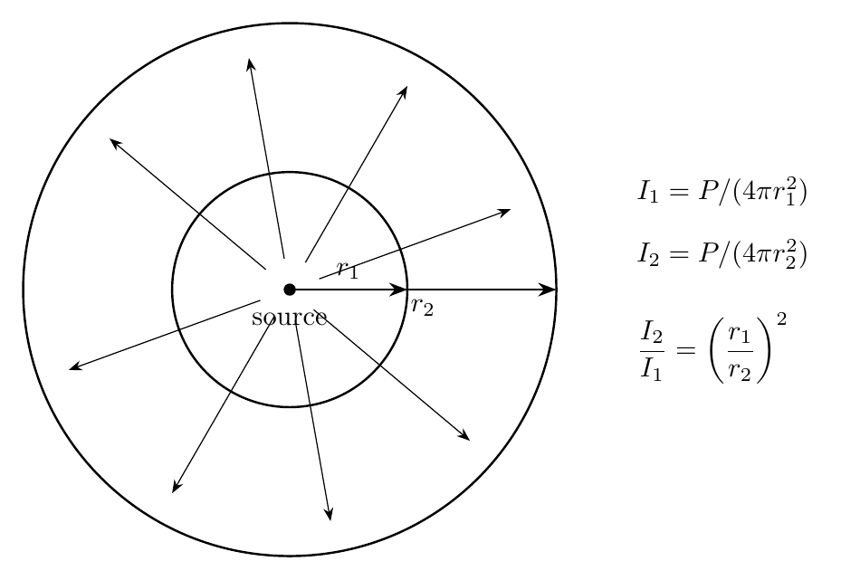
Figure. For lossless spherical spreading, the same source power crosses every spherical wavefront.

Exercise 6: Infer source power from a measured intensity

An ideal isotropic source produces intensity

I = 0.12 W ∕m2

(17)

at radius

r = 3.0m.

(18)

Find the source power.

Exercise 7: Geometric spreading or dissipation?

A wave has intensity

I1 = 0.10W ∕m2

(19)

at radius

r1 = 3.0m.

(20)

At radius

r2 = 8.0m,

(21)

its measured intensity is

I2 = 0.010W ∕m2.

(22)

Assume spherical wavefronts.

What would I₂ be for lossless geometric spreading alone?
What fraction of the power crossing the inner sphere remains at the outer sphere?
What fraction has been removed from the propagating wave?

Exercise 8: Identify the spreading geometry

The following figure summarizes three idealized spreading geometries.

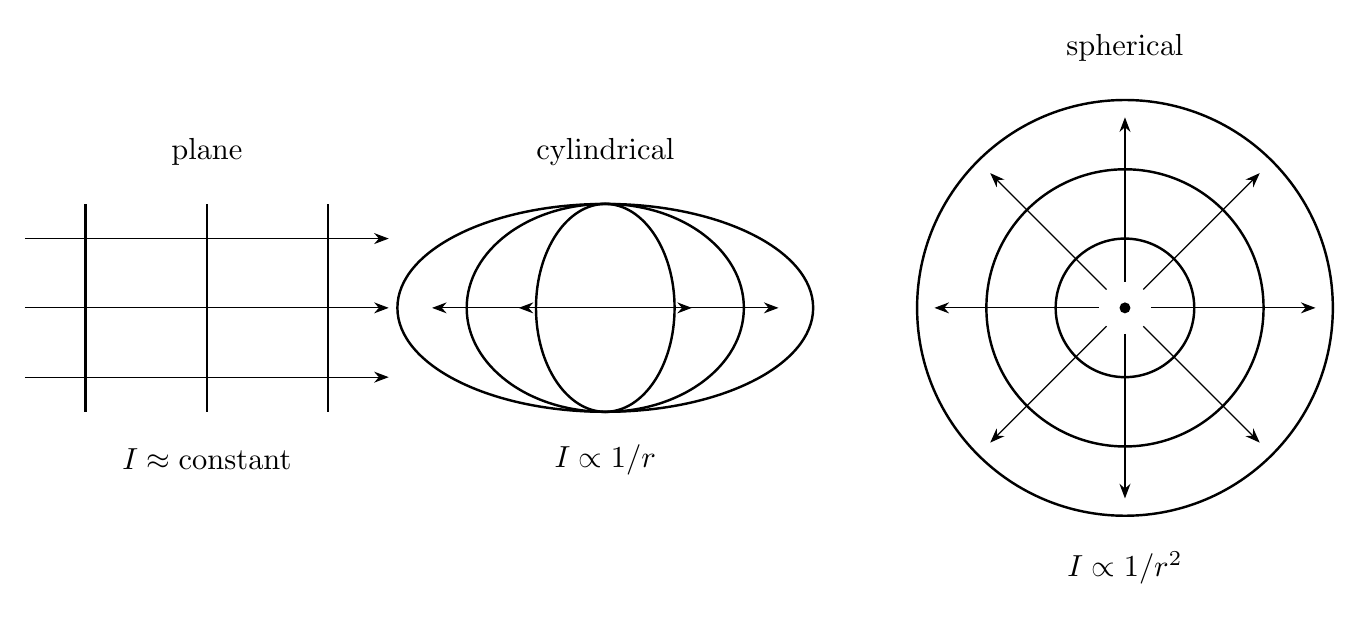
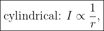
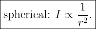
Figure. Ideal plane, cylindrical, and spherical spreading lead to different intensity laws.

Match each intensity law to its idealized spreading geometry:

1 1 I ≈ constant, I ∝ -, I ∝ -2. r r

(23)

Then explain why the inverse-square law is not universal for every wave.

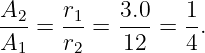
Exercise 9: Amplitude change for spherical spreading

A linear spherical wave has amplitude A₁ at radius

r = 3.0m. 1

(24)

Assume

2 I ∝ A

(25)

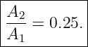
and lossless spherical spreading. Find A₂∕A₁ at

r2 = 12m.

(26)

Exercise 10: Local conservation of energy

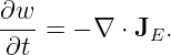
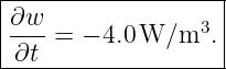
At a certain point in a three-dimensional wave field,

∇ ⋅ J = +4.0 W ∕m3. E

(27)

Use

∂w-+ ∇ ⋅ J = 0 ∂t E

(28)

to determine ∂w∕∂t. Explain the physical meaning of its sign.

Exercise 11: Bridge from string power to an effective intensity

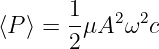
A sinusoidal wave on an ideal string has

μ = 0.010 kg/m, c = 80 m/s,

(29)

A = 1.5 mm, f = 50 Hz.

(30)

Use
$1 2 2 ⟨P ⟩ = -μA ω c 2$ (31)

to find the average string power.
If, only as a dimensional bridge, that power is uniformly distributed over an effective area
$Ae ff = 2.0 × 10−4m2,$ (32)

find the corresponding intensity.
Explain why the ideal 1D string itself does not intrinsically possess a unique areal intensity.

Exercise 12: Surface orientation

A uniform flux vector has magnitude

JE = 30W ∕m2.

(33)

A detector has area

A = 0.20m2.

(34)

Find the power crossing the detector when the angle between the flux and the detector normal is

0^∘,
60^∘,
90^∘.

Explain physically why the last answer is zero.

Exercise 13: Diagnose conceptual statements

Decide whether each statement is correct. If it is incorrect, rewrite it accurately.

“If intensity decreases with distance, wave energy must have been dissipated.”
“Intensity and power have the same SI units.”
“For an ideal isotropic source, doubling distance reduces intensity by a factor of four.”
“For a progressive nondispersive wave, I = c⟨w⟩.”
“The inverse-square law applies to every wave, independent of geometry.”
“Flux is fundamentally directional even when intensity is quoted as a positive scalar.”

Exercise 14: Synthesis problem

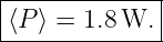
An ideal isotropic source radiates average power

Psource = 24 W.

(35)

The wave speed is

c = 300 m/s.

(36)

At radius

r1 = 4.0m,

(37)

answer the following.

Find the intensity.
Find the average volume energy density.
A perpendicular detector of area 0.030 m² is placed there. Find the average power crossing it.
Find the intensity at r₂ = 12 m.
If the wave is linear and I ∝ A², find the amplitude ratio A₂∕A₁ between the two radii.
State which parts of the intensity decrease are explained purely by geometry.

Part II: Complete Worked Solutions

Solution 1: Convert power to intensity

Use

I = ⟨P⟩. A

(38)

Therefore

I	= W∕m²	(39)
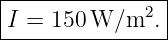
	= 150 W∕m².	(40)

Thus

----------------- | 2 | I-=-150-W-∕m--.--

(41)

The units are watts per square meter because intensity is power divided by area.

Solution 2: Same power, different area

For conserved power,

I A = I A . 1 1 2 2

(42)

Since

A2 = 4A1,

(43)

we have

A1- I1 I2 = I1A2 = 4 .

(44)

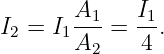
Therefore

|I----1--| |-2 = --.| -I1---4--|

(45)

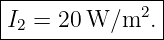
With I₁ = 80 W∕m²,

|------------2-| I2-=-20-W-∕m--.-

(46)

The decrease does not by itself imply dissipation. The same power can simply be spread over a larger area.

Solution 3: Flux through a tilted surface

For uniform flux,

P = JEA cosα.

(47)

Substitute the data:

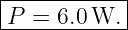
P	= (18)(0.60) cos 60^∘ W	(48)
	= (18)(0.60)(0.5) W	(49)
	= 5.4 W.	(50)

Hence

|-----------| P--=-5.4W.---

(51)

Only the normal component of the flux crosses the surface.

Solution 4: Intensity from volume energy density

For a progressive nondispersive wave,

I = c⟨w ⟩.

(52)

Therefore

I	= (250)(0.024) W∕m²	(53)
	= 6.0 W∕m².	(54)

Thus

|--------------| I = 6.0 W ∕m2. | ----------------

(55)

The power through 0.30 m² is

⟨P⟩ = IA = (6.0)(0.30 ) = 1.8 W.

(56)

Therefore

|-------------| ⟨P ⟩ = 1.8W. | --------------

(57)

Solution 5: Spherical spreading ratio

For lossless spherical spreading,

I ( r )2 -2 = -1 . I1 r2

(58)

Thus

I₂	= 0.36² W∕m²	(59)
	= 0.0576 W∕m².	(60)

Hence

|------------------------| |I2 = 5.76 × 10−2W ∕m2. | -------------------------

(61)

Solution 6: Infer source power from a measured intensity

From

I = Psource, 4πr2

(62)

solve for source power:

2 Psource = I4πr .

(63)

Therefore

P_source	= (0.12)4π(3.0)² W	(64)
	≃ 13.6 W.	(65)

Thus

|----------------| Psource ≃ 13.6 W.| ------------------

(66)

Solution 7: Geometric spreading or dissipation?

For lossless spherical spreading,

( )2 I = I r1 . 2,geom 1 r2

(67)

Thus

I_2,geom	= 0.10²	(68)
	= 0.0141 W∕m²	(69)

approximately.

The power through a spherical wavefront is

P = I4πr2.

(70)

Therefore the remaining power fraction is

	=	(71)
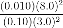	=	(72)
	≃ 0.711.	(73)

Hence

|------| -71.1%--

(74)

of the inner-sphere power remains. The removed fraction is

1 − 0.711 = 0.289,

(75)

|------| -28.9%--

(76)

has been removed from the propagating wave by effects beyond ideal geometric spreading.

Solution 8: Identify the spreading geometry

The idealized correspondences are

|--------------------| |plane: I ≈ constant,| ----------------------

(77)

|------------------| | 1-| |cylindrical: I ∝ r,| --------------------

(78)

and

|------------------| | 1- | |spherical: I ∝ r2.| -------------------

(79)

The inverse-square law is therefore not a universal wave law. It follows specifically from the growth of spherical wavefront area as 4πr².

Solution 9: Amplitude change for spherical spreading

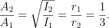
For a linear wave in a fixed medium,

2 I ∝ A .

(80)

For lossless spherical spreading,

I ∝ -1 . r2

(81)

Therefore

1- A ∝ r.

(82)

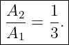
Hence

A2 r1 3.0 1 ---= -- = --- = -. A1 r2 12 4

(83)

Thus

|-----------| |A2-= 0.25. | |A1 | ------------

(84)

The amplitude becomes one quarter as large while the intensity becomes one sixteenth as large.

Solution 10: Local conservation of energy

The local conservation law is

∂w- = − ∇ ⋅ JE. ∂t

(85)

Given

∇ ⋅ JE = +4.0 W ∕m3,

(86)

we obtain

|------------------| |∂w- 3 | |∂t = − 4.0 W ∕m .| --------------------

(87)

The positive divergence means more energy is flowing out of the local volume than into it. Therefore the stored energy density decreases with time.

Solution 11: Bridge from string power to an effective intensity

First compute

ω = 2πf = 100π rad/s.

(88)

Then

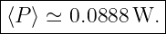
⟨P⟩	= μA²ω²c	(89)
	= (0.010)(1.5 × 10⁻³)²(100π)²(80)	(90)
	≃ 8.88 × 10⁻² W.	(91)

Thus

|----------------| |⟨P ⟩ ≃ 0.0888 W. | ------------------

(92)

The effective intensity is

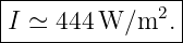
I	=	(93)
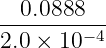	=	(94)
	≃ 4.44 × 10² W∕m².	(95)

Therefore

|------------2--| I-≃-444-W-∕m--.--

(96)

The ideal 1D string model intrinsically supplies energy per unit length and power through a point. It does not define a physical cross-sectional wavefront area over which that power is distributed. An areal intensity can therefore be assigned only after an area is introduced as an additional modeling assumption.

Solution 12: Surface orientation

Use

P = JEA cosα.

(97)

The product J_EA is

(30)(0.20) = 6.0W.

(98)

Therefore

For α = 0^∘,
$|-----------| P = 6.0W. | -------------$ (99)
For α = 60^∘,
$P = (6.0)(0.5) = |3.0W.--| --------|$ (100)
For α = 90^∘,
$|------| P--=-0.-$ (101)

At 90^∘, the flux is parallel to the detector surface, so no energy crosses through the surface normal direction.

Solution 13: Diagnose conceptual statements

Incorrect. Intensity can decrease because of geometric spreading even when the total wave power is conserved.
Incorrect. Power is measured in watts, while intensity is measured in watts per square meter.
Correct for an ideal isotropic source in three dimensions: doubling distance multiplies intensity by (1∕2)² = 1∕4.
Correct for a progressive nondispersive wave when w is the appropriate volume energy density.
Incorrect. The inverse-square law follows from spherical spreading. Plane and cylindrical geometries have different distance dependence.
Correct. The energy-flux vector carries direction. A scalar intensity normally reports the positive magnitude of the average flux in the propagation direction.

Solution 14: Synthesis problem

The source power is

Psource = 24 W.

(102)

At r₁ = 4.0 m,

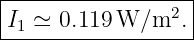
I₁	=	(103)
	≃ 0.119 W∕m².	(104)

Thus

|------------------| |I1 ≃ 0.119W ∕m2. | -------------------

(105)

For a progressive nondispersive wave,

⟨w⟩ = I1. c

(106)

Therefore

⟨w⟩	=	(107)
	≃ 3.98 × 10⁻⁴ J∕m³.	(108)

Hence

|------------------------| |⟨w⟩ ≃ 3.98 × 10− 4J∕m3. | -------------------------

(109)

The detector power is

⟨P_det⟩	= I₁A	(110)
	= (0.119)(0.030)	(111)
	≃ 3.58 × 10⁻³ W.	(112)

Thus

|------------------| |⟨Pdet⟩ ≃ 3.58 mW. | --------------------

(113)

At r₂ = 12 m,

( ) 4.0 2 I2 = I1 --- . 12

(114)

Therefore

-------------------- | 2 | I2-≃-0.0133-W-∕m--.-

(115)

Since I ∝ A² for the stated linear wave,

∘ --- A2- = I2= r1 = 1-. A1 I1 r2 3

(116)

Thus

|--------| |A2- 1-| |A = 3.| --1-------

(117)

Under the assumptions of the problem, the entire decrease from I₁ to I₂ is explained by geometric spreading. The same source power is distributed over the larger spherical area 4πr²; no dissipation was introduced.

Common mistakes

Mistake: using watts per square meter for power. Those are intensity units; power itself is measured in watts.
Mistake: concluding that every intensity decrease represents absorption. Geometric spreading can reduce intensity with no loss of total power.
Mistake: forgetting the cosine factor for a tilted receiving surface.
Mistake: applying I = cw to an arbitrary standing or multidirectional field without checking whether a single progressive transport velocity is appropriate.
Mistake: applying 1∕r² to plane or cylindrical waves.
Mistake: assigning an intrinsic areal intensity to a 1D string without defining an area.

What WM21E1 reinforces

This exercise set reinforces the hierarchy

|----------------------------------| -energy-−→--power-−-→--flux-density.-

(118)

The same physical conservation idea appears in different dimensional forms:

ℰt + Px = 0

(119)

for the 1D string and

∂w- ∂t + ∇ ⋅ JE = 0

(120)

for a multidimensional field. The geometry of the wavefront then determines how a fixed total power is distributed in space.

References

[1] A. P. French, Vibrations and Waves, M.I.T. Introductory Physics Series, W. W. Norton & Company, 1971.

[2] Frank S. Crawford, Jr., Waves, Berkeley Physics Course, Volume 3, McGraw-Hill, 1968.

[3] William Moebs, Samuel J. Ling, and Jeff Sanny, University Physics, Volume 1, OpenStax, 2016, Section 16.4, “Energy and Power of a Wave.”

[4] William Moebs, Samuel J. Ling, and Jeff Sanny, University Physics, Volume 1, OpenStax, 2016, Section 17.3, “Sound Intensity.”

[5] Massachusetts Institute of Technology, 8.03SC Physics III: Vibrations and Waves, MIT OpenCourseWare, Fall 2016.

[6] Massachusetts Institute of Technology, 2.24 / 13.022 Ocean Wave Interaction with Ships and Offshore Energy Systems, Lecture 4, “Wave Energy Density and Flux,” MIT OpenCourseWare, Spring 2002.

"example of Wave Mechanics: Wave Intensity and Flux" is owned by bloftin.
(view preamble)