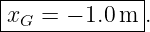
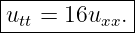
Wave Mechanics Examples: Right- and Left-Traveling Solutions
This companion article provides exercises for WM16, wave mechanics: Right- and Left-Traveling
Solutions. All exercises are stated first so they can be attempted without seeing the answers.
Complete worked solutions follow in Part II.
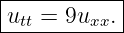
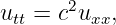
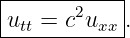
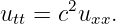
The central WM16 result is that, for a sufficiently smooth classical solution of the homogeneous
one-dimensional constant-speed wave equation,
one may write
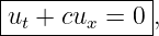
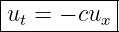
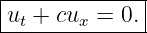
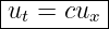
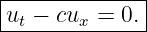
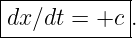
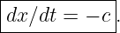
The two pure traveling families satisfy the first-order transport relations
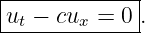
and
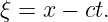
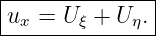
The characteristic variables are
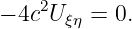
and in these coordinates the wave equation reduces to
These results are standard descriptions of the one-dimensional wave equation and traveling-wave
decomposition [1, 2, 3, 4, 6].
How to use this problem set
For each problem, separate three questions:
- which part of the field moves toward +x and which part moves toward −x;
- what information follows from the second-order wave equation itself; and
- what extra information requires initial or boundary data.
The distinction between a pure one-way wave and a superposition containing both families is
especially important.
Part I: Exercises
Exercise 1: Read the two propagation families from snapshots
The figure below shows the same localized profile at an earlier and a later time for each traveling
family.
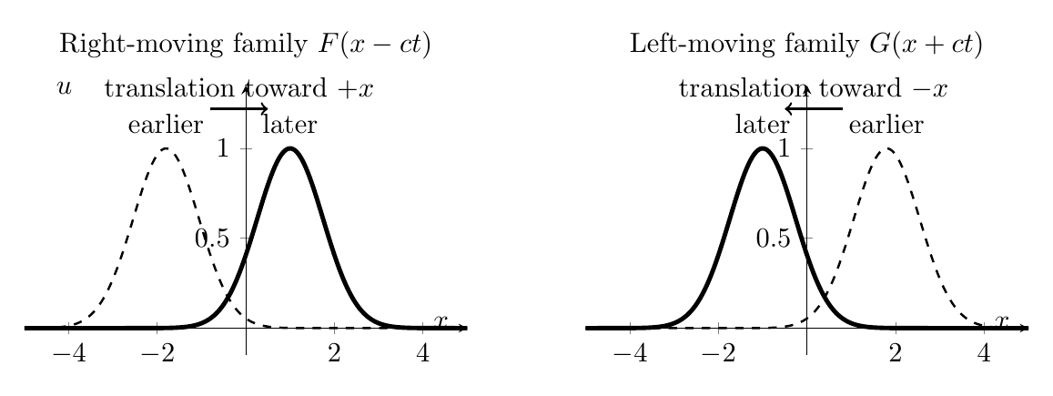
Figure. A profile depending on x − ct translates toward increasing x, while a profile
depending on x + ct translates toward decreasing x.
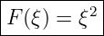
- Which panel represents F(x − ct)?
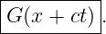
- Which panel represents G(x + ct)?
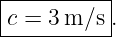
- If the peak in the right-moving panel shifts by 2.8 m during 0.70 s, find c.
- Write the first-order transport equation satisfied by each pure family.
Exercise 2: Derive and use the first-order direction tests
For
and
derive the relation between ut and ux for each family.
Then suppose a known pure one-way wave has, at one event,
Determine its direction and speed.
Exercise 3: Factor the wave operator
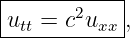
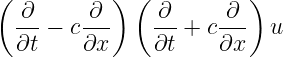
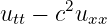
Expand
and show that it equals
for a sufficiently smooth function u(x,t). State precisely which derivative identity makes the two
mixed terms cancel.
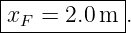
Exercise 4: Read characteristic footpoints
The figure shows the two characteristic lines through an event P = (x0,t0).
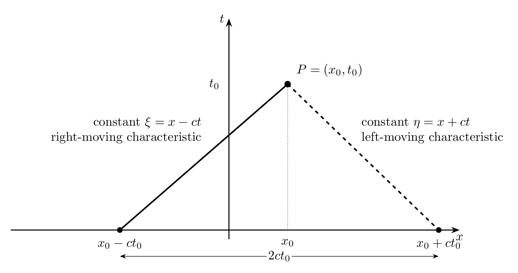
Figure. The two characteristics through P meet the initial line t = 0 at x0 − ct0 and
x0 + ct0.
Take
- Find the initial-line point on the constant-ξ characteristic.
- Find the initial-line point on the constant-η characteristic.
- Find the separation between the two footpoints.
- Which characteristic family has slope dx∕dt = +c?
- Which has slope dx∕dt = −c?
Exercise 5: Transform the wave equation
Let
Derive
and
Then derive uxx and utt and show that
What equation must U satisfy when c≠0?
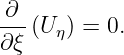
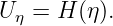
Exercise 6: Integrate the characteristic-coordinate equation
Starting from
integrate carefully to show that
Explain why the “constant of integration” after integrating with respect to η may be an arbitrary
function of ξ rather than an ordinary numerical constant.
Exercise 7: Identify the two components in a compound field
Consider
- Identify a possible F(ξ) and G(η).
- State the direction of each component.
- Find the common wave-speed magnitude.
- State the wave equation satisfied by the total field.
- Find the position of the center of the Gaussian component as a function of time.
Exercise 8: Point-by-point addition of the two families
At one instant, suppose the two traveling components are
and
The corresponding component profiles and their sum are shown below.
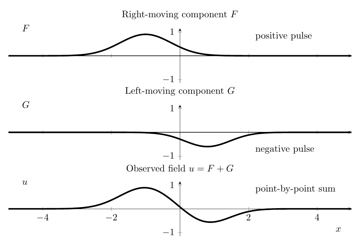
Figure. The observed displacement is the point-by-point sum of the right-moving and
left-moving components.
- Evaluate F(0).
- Evaluate G(0).
- Find u(0) = F(0) + G(0).
- Explain why destructive interference at one location does not mean the two traveling
components cease to exist.
Exercise 9: Decompose a non-obvious polynomial solution
Show that
satisfies
Then use the identity
to write the solution explicitly as
Exercise 10: Reconstruct a standing wave from two traveling families
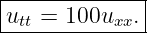
A Standing Wave is
where x is in meters and t is in seconds.
The figure illustrates the decomposition conceptually.
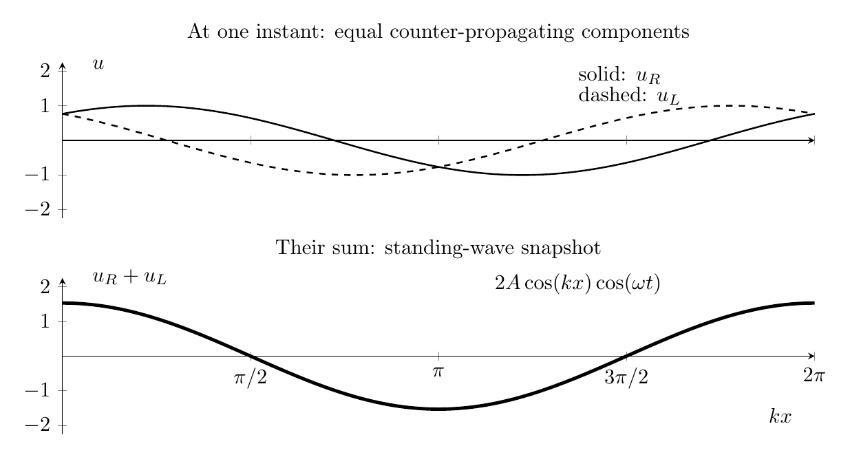
Figure. Equal counter-propagating sinusoidal components combine into a standing-wave
snapshot.
- Use a trigonometric identity to write u as the sum of one right-moving and one
left-moving sinusoid.
- What is the amplitude of each traveling component?
- Find k, ω, and the common wave speed c.
- State the wave equation satisfied by the standing wave.
Exercise 11: Why the pure transport tests fail for a two-way field
Let
Derive ux and ut, and then show that
and
Explain why a general two-way field normally satisfies neither pure first-order transport equation
even though it satisfies the second-order wave equation.
Exercise 12: Characteristic reach back to the initial line
At the event
let
- Find x0 − ct0.
- Find x0 + ct0.
- What interval of the initial line lies between those two characteristic footpoints?
- Why is this construction useful when initial data are eventually used to determine F
and G?
Exercise 13: Connect string mechanics to the two traveling families
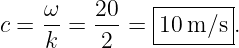
An ideal string has
A sinusoidal component has
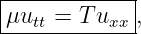
- Find the wave speed c.
- Find the angular frequency ω.
- Write a right-moving sinusoid of amplitude 3.0 mm and zero phase constant.
- Write the corresponding left-moving sinusoid.
- State the mechanical wave equation in both T,μ form and c form.
Exercise 14: Synthesis - two pulses and their initial data
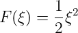
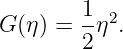
Let
and
Take
and define
- Write the complete function u(x,t) explicitly.
- State the propagation direction of each pulse.
- Write the initial displacement u(x, 0).
- Compute the initial velocity ut(x, 0).
- At t = 0.50 s, locate the center of each pulse.
- State the wave equation satisfied by u and explain why no direct second-derivative
calculation is needed to establish it.
Part II: Complete Worked Solutions
Solution 1: Read the two propagation families from snapshots
- The left panel moves toward increasing x, so it represents
- The right panel moves toward decreasing x, so it represents
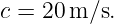
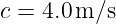
- The speed magnitude is displacement divided by elapsed time:
| c | =  | (40)
|
| = 4.0 m/s . | (41) |
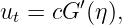
- The pure right-moving family satisfies
while the pure left-moving family satisfies
Solution 2: Derive and use the first-order direction tests
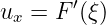
For the right-moving family, let
Then
and
Therefore
or
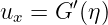
For the left-moving family, let
Then
and
so
or
For the measured event,
The two derivatives have opposite signs, which is consistent with the right-moving relation. Solving
for c,
| c | = − | (55)
|
| = − m/s m/s | (56)
|
| = 60 m/s . | (57) |
Thus the wave is purely right-moving at speed 60 m/s under the stated one-way-wave
assumption.
Solution 3: Factor the wave operator
Expand the two operators in order:
| 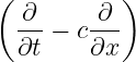 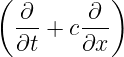 u u | (58)
|
| = 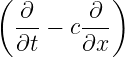  | (59)
|
| = utt + cuxt − cutx − c2u
xx. | (60) |
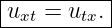
For a sufficiently smooth function, the mixed partial derivatives commute:
Therefore the middle terms cancel and
This factorization exposes the two first-order propagation operators hidden inside the second-order
wave equation.
Solution 4: Read characteristic footpoints
We have
First compute
- The constant-ξ characteristic reaches the initial line at
| x0 − ct0 | = 5.0 − 2.0 | (65)
|
| = 3.0 m . | (66) |
- The constant-η characteristic reaches the initial line at
| x0 + ct0 | = 5.0 + 2.0 | (67)
|
| = 7.0 m . | (68) |
- Their separation is
- Constant ξ = x − ct gives
so
- Constant η = x + ct gives
so
Solution 5: Transform the wave equation
Let
Because
the chain rule gives
Differentiate once more with respect to x:
Similarly,
so
Differentiating again with respect to t gives
Subtracting c2u
xx,
| utt − c2u
xx | = c2U
ξξ − 2c2U
ξη + c2U
ηη | (81)
|
| − c2 | (82)
|
| = −4c2U
ξη. | (83) |
Thus the wave equation requires
For c≠0,
Solution 6: Integrate the characteristic-coordinate equation
Start from
Write this as
Therefore Uη does not depend on ξ. It may still depend on η, so write
Integrating with respect to η gives
The term F(ξ) appears because integration was performed with respect to η. Anything that
depends only on ξ differentiates to zero with respect to η, so it plays the role of an integration
constant.
Therefore
and hence
Solution 7: Identify the two components in a compound field
The field is
Define
Then one valid choice is
and
The F component moves toward increasing x and the G component moves toward decreasing x.
Both have speed magnitude
Therefore the total field satisfies
The Gaussian is centered when its squared argument vanishes:
Hence its center is
The decreasing center position confirms leftward propagation.
Solution 8: Point-by-point addition of the two families
At x = 0,
| F(0) | = 0.90e−0.9(1)2
| (100)
|
| ≈ 0.366 . | (101) |
For the second component,
| G(0) | = −0.60e−1.15(−0.8)2
| (102)
|
| = −0.60e−0.736 | (103)
|
| ≈−0.287 . | (104) |
Therefore
| u(0) | = F(0) + G(0) | (105)
|
| ≈ 0.366 − 0.287 | (106)
|
| ≈ 0.0785 . | (107) |
The two components partially cancel at this location, but the linear wave model still contains both
traveling contributions. Interference changes their observed sum; it does not destroy the underlying
component solutions.
Solution 9: Decompose a non-obvious polynomial solution
For
we have
and
Thus
so the wave equation is satisfied.
Now use
Dividing by 2,
Therefore choose
and
Hence
This again shows that the two-family representation is not limited to pulses and sinusoids.
Solution 10: Reconstruct a standing wave from two traveling families
The standing wave is
Use
Then
| u | = 4.0 mm cos(2x − 20t) | (119)
|
| + 4.0 mm cos(2x + 20t). | (120) |
Thus
and
Each component amplitude is therefore
The Wavenumber and angular frequency are
Hence
The wave equation is therefore
Solution 11: Why the pure transport tests fail for a two-way field
Let
For
we obtain
and
Therefore
| ut + cux | = ![[− cF ′ + cG ′]](https://images.physicslibrary.org/cache/objects/1180/make4ht/ExampleOfWaveMechanicsRightAndLeftTravelingSolutions113x.png) + c + c![[F ′ + G ′]](https://images.physicslibrary.org/cache/objects/1180/make4ht/ExampleOfWaveMechanicsRightAndLeftTravelingSolutions114x.png) | (131)
|
| = 2cG′(η) . | (132) |
Likewise,
| ut − cux | = ![[− cF ′ + cG ′]](https://images.physicslibrary.org/cache/objects/1180/make4ht/ExampleOfWaveMechanicsRightAndLeftTravelingSolutions115x.png) − c − c![[F ′ + G ′]](https://images.physicslibrary.org/cache/objects/1180/make4ht/ExampleOfWaveMechanicsRightAndLeftTravelingSolutions116x.png) | (133)
|
| = −2cF′(ξ) . | (134) |
Thus the right-moving transport equation ut + cux = 0 holds for the total field only where the
left-moving derivative contribution vanishes. Similarly, ut − cux = 0 holds only where the
right-moving derivative contribution vanishes.
A general two-way field therefore satisfies the second-order wave equation but normally satisfies
neither pure one-way first-order transport equation.
Solution 12: Characteristic reach back to the initial line
At
we have
Therefore
and
The interval between the footpoints is
The two characteristics show where the two traveling families reaching the event P trace back to
the initial line. In WM17, initial displacement and velocity data will be used to determine the
specific functions F and G, and these characteristic locations will enter naturally into the resulting
formula.
Solution 13: Connect string mechanics to the two traveling families
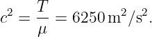
For an ideal string,
Therefore
| c | =  | (141)
|
| =  | (142)
|
| ≈ 79.1 m/s . | (143) |
With
the nondispersive relation gives
| ω | = ck | (145)
|
| = (79.1)(5.0) | (146)
|
| ≈ 395 rad/s . | (147) |
A right-moving sinusoid with amplitude 3.0 mm is
The corresponding left-moving sinusoid is
The mechanical form of the string equation is
or equivalently
Here
Solution 14: Synthesis - two pulses and their initial data
The two profile functions are
and
with
- Substitute s = x − 4t into F and s = x + 4t into G:
- The first pulse depends on x − 4t, so it moves toward +x. The second depends on x + 4t, so
it moves toward −x.
- At t = 0,
- For the general two-family form,
Here
and
Therefore at t = 0,
- The first pulse is centered where
so at t = 0.50 s,
The second pulse is centered where
giving
- Each component is a sufficiently smooth function of one characteristic variable, and the wave
equation is linear. Therefore the sum satisfies
No fresh second-derivative calculation is required because the WM15 verification theorem
and linearity already establish the result.
Common mistakes
- Mistake: reading the sign inside x ∓ ct as the direction itself. Direction comes from
holding the whole argument constant.
- Mistake: applying ut = −cux or ut = cux to a field that contains both traveling
families.
- Mistake: forgetting that factorization uses differential operators and requires
commuting mixed partial derivatives for the classical derivation.
- Mistake: treating the integration function F(ξ) as an ordinary numerical constant
when integrating with respect to η.
- Mistake: assuming F and G have been determined merely because the PDE has been
solved structurally. Initial or boundary data are still required.
- Mistake: assuming a standing wave is unrelated to traveling waves. It can be built
from equal counter-propagating components.
What WM16E1 reinforces
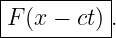
The one-dimensional constant-speed wave equation contains two independent characteristic
propagation families. In characteristic coordinates,
the second-order equation reduces to
whose sufficiently smooth solutions have the form
WM17 will use initial displacement and initial velocity to determine the specific functions F and G
and obtain the d’Alembert initial-value formula.
References
References
[1] A. P. French, Vibrations and Waves, M.I.T. Introductory Physics Series, W. W.
Norton & Company, 1971.
[2] Frank S. Crawford, Jr., Waves, Berkeley Physics Course, Volume 3, McGraw-Hill,
1968.
[3] William Moebs, Samuel J. Ling, and Jeff Sanny, University Physics, Volume 1,
OpenStax, 2016, Section 16.2, “Mathematics of Waves.”
[4] Richard P. Feynman, Robert B. Leighton, and Matthew Sands, The Feynman Lectures
on Physics, Volume I, Chapter 47, “Sound. The Wave Equation.”
[5] Richard P. Feynman, Robert B. Leighton, and Matthew Sands, The Feynman Lectures
on Physics, Volume I, Chapter 48, “Beats.”
[6] Massachusetts Institute of Technology, 8.03SC Physics III: Vibrations and Waves,
Lecture 10, “Traveling Waves,” MIT OpenCourseWare.

![[parent]](https://images.physicslibrary.org/images/uparrow.png)















![[ ]
u(x,t) = (x − 3t)2 + 0.40 exp − (x + 3t − 1)2 .](https://images.physicslibrary.org/cache/objects/1180/make4ht/ExampleOfWaveMechanicsRightAndLeftTravelingSolutions18x.png)



































![[ ]
u(x,t) = (x − 3t)2 + 0.40 exp − (x + 3t − 1)2 .](https://images.physicslibrary.org/cache/objects/1180/make4ht/ExampleOfWaveMechanicsRightAndLeftTravelingSolutions84x.png)