Wave Mechanics Examples: Initial Conditions and the d’Alembert Solution
This companion article provides exercises for WM17, wave mechanics: Initial Conditions and the
d’Alembert Solution. All exercises are stated first so they can be attempted without seeing the
answers. Complete worked solutions follow in Part II.
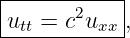
For the one-dimensional constant-speed wave equation on the whole line,
with initial data
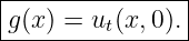
and
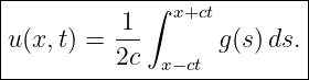
the d’Alembert formula is
The first term carries the initial displacement along the two characteristic directions. The integral
term carries the effect of the initial velocity over the characteristic interval. This is
the classical whole-line initial-value solution under the usual smoothness assumptions
[4, 3, 6].
How to use this problem set
Attempt all exercises in Part I before consulting Part II. In each problem, identify the
characteristic endpoints
before substituting into the formula. Keep the whole-line assumption in mind: a finite string
also requires endpoint boundary conditions and generally involves reflections or mode
expansions.
Part I: Exercises
Exercise 1: Read the d’Alembert formula
Consider
Answer the following.
- Which function represents the initial displacement?
- Which function represents the initial velocity?
- What are the two characteristic footpoints on the line t = 0?
- Which part of the formula survives if g(x) = 0?
- Which part survives if f(x) = 0?
Exercise 2: Released displacement with zero initial velocity
Suppose
- Simplify the d’Alembert formula.
- Explain why the initial profile splits into two copies.
- What is the amplitude of each copy relative to the original amplitude?
- What direction does each copy move?
- Show explicitly that the two copies add back to f(x) at t = 0.
The geometry is illustrated below.

Figure. With zero initial velocity, the initial displacement separates into equal right- and
left-moving half-amplitude copies.
Exercise 3: Initial velocity required for one-way motion
An initial shape f(x) is prescribed.
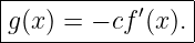
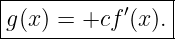
- What initial velocity g(x) produces a pure right-moving solution?
- What initial velocity produces a pure left-moving solution?
- For
find g(x) for pure right-moving motion.
- For the same f(x), find g(x) for pure left-moving motion.
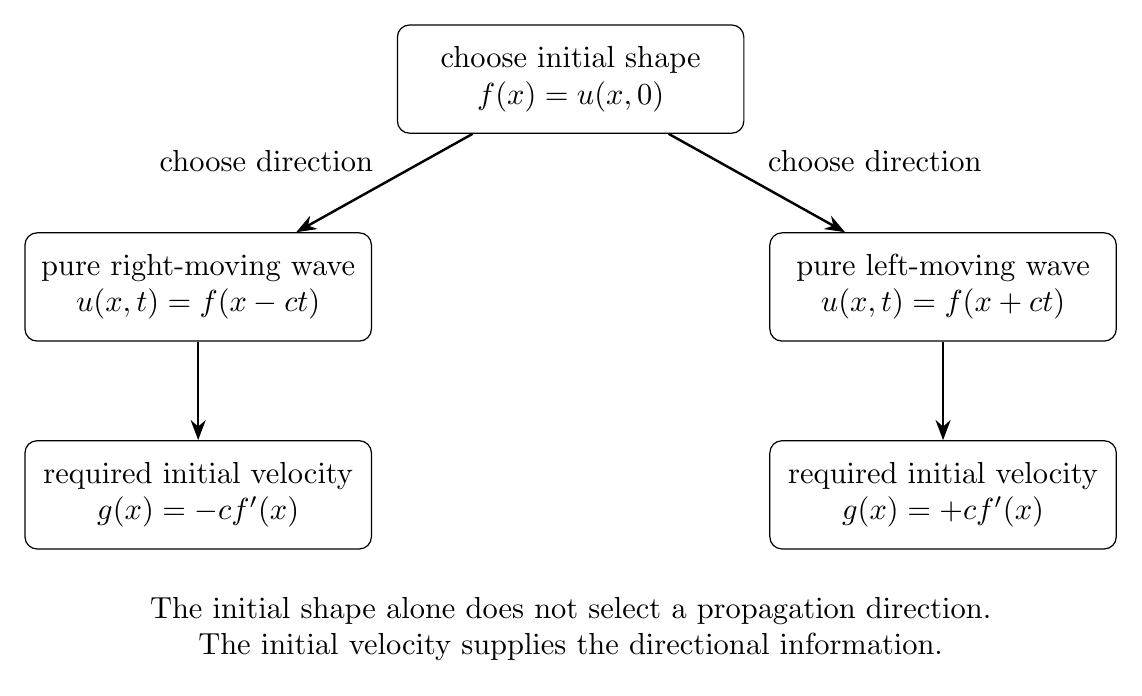
Figure. The initial displacement alone does not determine propagation direction. The
initial velocity carries the directional information.
Exercise 4: Recover the two traveling components
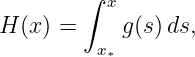
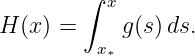
Define
where x∗ is a fixed reference point.
Starting from
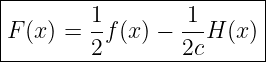
show that one convenient choice of the component functions is
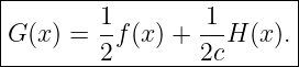
and
Explain why adding a constant to F and subtracting the same constant from G does not change
u(x,t).
Exercise 5: Direct numerical evaluation
Let
and let the initial data be
Find
Show separately the displacement contribution and the initial-velocity contribution.
Exercise 6: Velocity-only compact pulse
Suppose the initial displacement is zero,
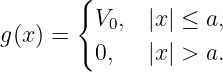
and the initial velocity is
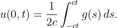
At the observation point x = 0:
- Find u(0,t) for 0 ≤ t ≤ a∕c.
- Find u(0,t) for t ≥ a∕c.
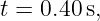
- Evaluate the result for
at t = 0.10 s and t = 0.30 s.
The integral is controlled by the overlap between the characteristic interval and the support of
g.
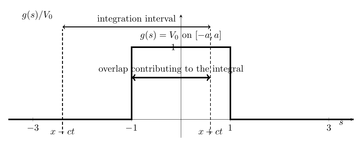
Figure. Only the portion of the initial-velocity profile inside [x − ct,x + ct] contributes to
the velocity integral.
Exercise 7: Sinusoidal initial displacement
Let
- Use the d’Alembert formula to find u(x,t).
- Use a trigonometric identity to simplify the result.
- Show that the angular frequency is ω = ck.
- Explain why the final expression is a standing-wave form even though d’Alembert’s
solution is built from traveling waves.
Exercise 8: Sinusoidal initial velocity
Let
- Evaluate the velocity integral.
- Show that
- Rewrite the coefficient using ω = ck.
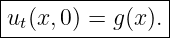
- Differentiate the result with respect to time and verify ut(x, 0) = g(x).
Exercise 9: Domain of dependence
At the observation point
suppose the wave speed is
- Find the two characteristic footpoints on the initial line.
- State the interval of initial data that can influence (x0,t0).
- Can a change in the initial data at x = 2.2 m influence the observation point?
- Can a change at x = 5.4 m influence it?
- Can a change at x = 6.0 m influence it?
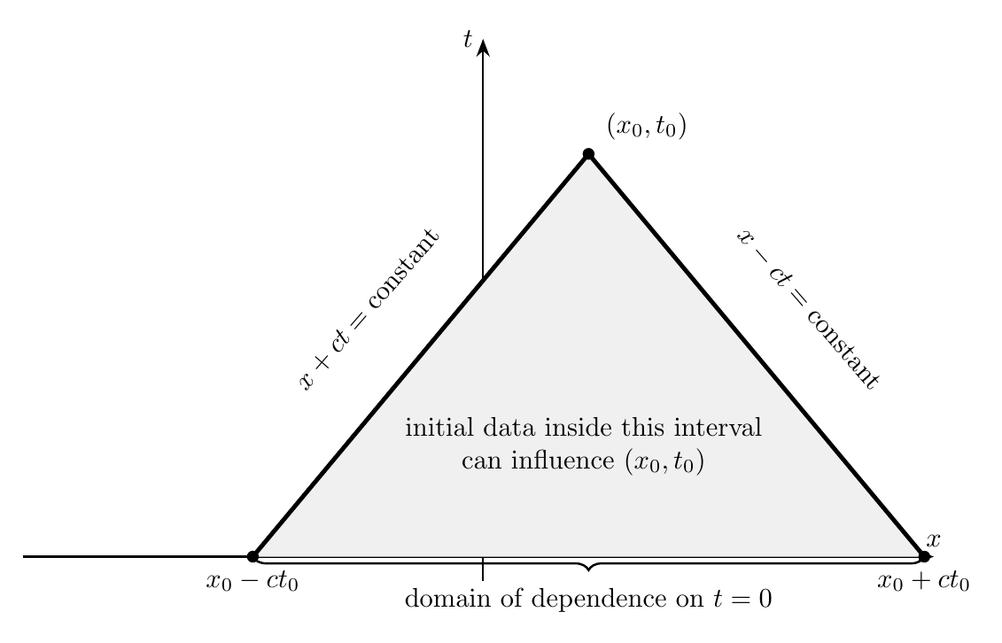
Figure. The point (x0,t0) depends only on initial data inside the interval [x0 −ct0,x0 +ct0].
Exercise 10: Finite propagation from compactly supported data
Suppose both initial functions vanish outside
The wave speed is
At time
find the largest interval in which the solution can possibly be nonzero. Explain how this
demonstrates finite propagation speed.
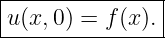
Exercise 11: Check the initial conditions directly
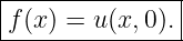
Starting from
show directly that
and
For the velocity check, use the Leibniz rule for differentiating an integral whose limits depend on
time.
Exercise 12: Whole-line formula versus a finite string
A string occupies only
and is fixed at both ends:
Answer the following.
- Does the basic whole-line d’Alembert formula automatically enforce these endpoint
conditions?
- What additional physical phenomenon appears when waves reach the endpoints?
- Name two methods that can be used to solve the finite-string problem after boundary
conditions are imposed.
- Explain why applying the whole-line formula blindly to a finite string can give the
wrong physical answer.
Exercise 13: Connect the initial-value solution to string mechanics
An ideal string has
The initial displacement is
and the initial velocity is zero.
- Find the wave speed.
- Write the complete d’Alembert solution.
- At t = 0.010 s, where are the centers of the two Gaussian pulses?
- What is the peak amplitude of each separated pulse?
Exercise 14: Synthesis – design a pure right-moving sinusoid
An ideal string has
The desired initial displacement is
The goal is for this entire shape to travel purely to the right.
- Find the wave speed c.
- Find the required initial velocity g(x).
- Write the resulting traveling-wave solution u(x,t).
- Identify k and ω.
- Find the wavelength and ordinary frequency.
- Explain why choosing g(x) = 0 instead would not produce the same motion.
Part II: Complete Worked Solutions
Solution 1: Read the d’Alembert formula
The formula is
- The initial displacement is
- The initial velocity is
- The characteristic footpoints are
- If g = 0, only the displaced copies of f remain:
- If f = 0, only the velocity integral remains:
Solution 2: Released displacement with zero initial velocity
Setting
removes the integral term, so
The first term is a right-moving copy because its argument is x − ct. The second is a left-moving
copy because its argument is x + ct.
Each copy has one-half the initial amplitude. At t = 0,
| u(x, 0) | =  f(x) + f(x) +  f(x) f(x) | (45)
|
| = f(x) . | (46) |
Thus the two half-amplitude copies exactly reconstruct the original profile at the initial
instant.
Solution 3: Initial velocity required for one-way motion
For a pure right-moving wave,
Differentiate with respect to time:
At t = 0,
Similarly, for a pure left-moving wave,
so
Now let
Then
Therefore the required right-moving initial velocity is
whereas the required left-moving initial velocity is
The sign of the initial velocity therefore selects the propagation direction.
Solution 4: Recover the two traveling components
WM17 gives
and
Define
Integrating gives one convenient choice,
and
Their sum is
as required by the initial displacement.
If a constant C is added to F and subtracted from G, then
Therefore the physical field u(x,t) is unchanged by this constant redistribution between the two
component functions.
Solution 5: Direct numerical evaluation
The observation event is
with
The characteristic endpoints are
| x − ct | = 1.0 − (2.5)(0.20) = 0.50 m, | (65)
|
| x + ct | = 1.0 + (2.5)(0.20) = 1.50 m. | (66) |
The displacement contribution is
 [f(0.50) + f(1.50)] [f(0.50) + f(1.50)] | =  α[(0.50)2 + (1.50)2] α[(0.50)2 + (1.50)2] | (67)
|
| =  (0.020)(0.25 + 2.25) m (0.020)(0.25 + 2.25) m | (68)
|
| = 0.025 m . | (69) |
The velocity contribution is
 ∫
0.501.50βsds ∫
0.501.50βsds | =  ![[s2 ]
--
2](https://images.physicslibrary.org/cache/objects/1182/make4ht/ExampleOfWaveMechanicsInitialConditionsAndTheDAlembertSolution69x.png) 0.501.50 0.501.50 | (70)
|
| =  ![[ ]
2.25 − 0.25
-----2-----](https://images.physicslibrary.org/cache/objects/1182/make4ht/ExampleOfWaveMechanicsInitialConditionsAndTheDAlembertSolution71x.png) m m | (71)
|
| = 0.060 m . | (72) |
Therefore
Solution 6: Velocity-only compact pulse
Because f = 0,
For early times with
the entire interval [−ct,ct] lies inside the region where g = V 0. Thus
| u(0,t) | =  V 0(2ct) V 0(2ct) | (76)
|
| = V 0t , 0 ≤ t ≤ . . | (77) |
For later times,
the integration interval already covers the full support [−a,a]. Hence
| u(0,t) | =  V 0(2a) V 0(2a) | (79)
|
| =  , t ≥ , t ≥ . . | (80) |
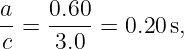
With
we have at t = 0.10 s,
At t = 0.30 s,
The plateau occurs because, after t = a∕c, expanding the characteristic interval does not include
any new region where g is nonzero.
Solution 7: Sinusoidal initial displacement
With
the d’Alembert formula becomes
Use
With
we obtain
The temporal factor has angular frequency
The result is a standing-wave form because equal right- and left-moving waves of the same
amplitude superpose to make a nontranslating pattern with fixed nodes and antinodes.
Solution 8: Sinusoidal initial velocity
Here
Therefore
Integrate:
| u(x,t) | =  ![[cos(kx − kct) − cos(kx + kct)]](https://images.physicslibrary.org/cache/objects/1182/make4ht/ExampleOfWaveMechanicsInitialConditionsAndTheDAlembertSolution93x.png) . . | (92) |
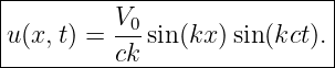
Using
we obtain
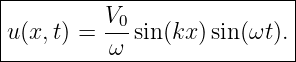
Since
this can be written as
Differentiate with respect to time:
At t = 0,
Solution 9: Domain of dependence
The characteristic endpoints are
| x0 − ct0 | = 4.0 − (5.0)(0.30) = 2.5 m, | (99)
|
| x0 + ct0 | = 4.0 + (5.0)(0.30) = 5.5 m. | (100) |
Therefore the domain of dependence on the initial line is
A change at x = 2.2 m lies outside this interval, so it cannot influence (x0,t0).
A change at x = 5.4 m lies inside the interval, so it can influence the observation point.
A change at x = 6.0 m lies outside the interval, so it cannot influence the observation
point.
Thus
Solution 10: Finite propagation from compactly supported data
Initially, both f and g vanish outside
In time t, information can propagate outward by at most the distance
Therefore the largest possible support at that time is
Hence
Outside this interval, neither characteristic reaching (x,t) can intersect nonzero initial data. The
disturbance therefore cannot appear arbitrarily far away instantly. This is finite propagation at
speed c.
Solution 11: Check the initial conditions directly
Start with
Set t = 0:
| u(x, 0) | =  [f(x) + f(x)] + [f(x) + f(x)] +  ∫
xxg(s) ds ∫
xxg(s) ds | (108)
|
| = f(x). | (109) |
Thus
Now differentiate with respect to time. The first two terms give
For the integral term, the Leibniz rule gives
 ![[ 1 ∫ x+ct ]
--- g(s)ds
2c x−ct](https://images.physicslibrary.org/cache/objects/1182/make4ht/ExampleOfWaveMechanicsInitialConditionsAndTheDAlembertSolution112x.png) | =  ![[cg(x + ct) + cg (x − ct)]](https://images.physicslibrary.org/cache/objects/1182/make4ht/ExampleOfWaveMechanicsInitialConditionsAndTheDAlembertSolution114x.png) | (112)
|
| =  [g(x + ct) + g(x − ct)]. [g(x + ct) + g(x − ct)]. | (113) |
Therefore
| ut(x,t) | = − f′(x − ct) + f′(x − ct) +  f′(x + ct) f′(x + ct) | (114)
|
| +  [g(x + ct) + g(x − ct)]. [g(x + ct) + g(x − ct)]. | (115) |
At t = 0, the two f′ terms cancel:
Hence
Solution 12: Whole-line formula versus a finite string
- No. The basic whole-line d’Alembert formula is constructed for an unbounded spatial
domain. It does not automatically impose
- When a wave reaches a finite endpoint, it reflects. The boundary condition determines the
reflected behavior.
- Two standard methods are reflected or extended initial data and normal-mode/Fourier-series
expansion.
- Applying the whole-line formula blindly would allow the wave to pass beyond the physical
endpoints instead of reflecting and satisfying the endpoint constraints. The resulting field
could therefore violate the actual boundary conditions.
Thus the whole-line formula solves an initial-value problem, while a finite string requires an
initial-boundary-value problem.
Solution 13: Connect the initial-value solution to string mechanics
For an ideal string,
With
we obtain
| c | =  | (121)
|
| =  | (122)
|
| ≈ 63.2 m/s . | (123) |
Because g = 0, the solution is
| u(x,t) | = 0.004 exp ![[ ( )2]
x −-ct
− 0.20](https://images.physicslibrary.org/cache/objects/1182/make4ht/ExampleOfWaveMechanicsInitialConditionsAndTheDAlembertSolution126x.png) | (124)
|
| + 0.004 exp ![[ ]
( x + ct)2
− ------
0.20](https://images.physicslibrary.org/cache/objects/1182/make4ht/ExampleOfWaveMechanicsInitialConditionsAndTheDAlembertSolution127x.png) m. m. | (125) |
At
the pulse centers are at
Therefore
Each separated pulse has one-half the initial peak amplitude:
Solution 14: Synthesis – design a pure right-moving sinusoid
The wave speed is
| c | =  | (130)
|
| =  | (131)
|
| =  | (132)
|
| = 40 m/s . | (133) |
The initial displacement is
Differentiate:
For pure right-moving motion,
Therefore
| g(x) | = −40[−0.030 sin(5x)] | (137)
|
| = 1.20 sin(5x) m/s . | (138) |
The complete right-moving solution is
Expanding the phase,
Hence
The wavelength is
| λ | =  | (142)
|
| =  | (143)
|
| ≈ 1.26 m . | (144) |
The ordinary frequency is
| fwave | =  | (145)
|
| =  | (146)
|
| ≈ 31.8 Hz . | (147) |
If instead g(x) = 0, the d’Alembert formula would produce
which is an equal two-way split, not a single right-moving waveform. The nonzero initial velocity is
what removes the unwanted left-moving component.
Common mistakes
- Mistake: forgetting that both f and g are required for a second-order-in-time wave
equation.
- Mistake: omitting the factor 1∕2 on the two displaced copies of f.
- Mistake: reversing the limits of the velocity integral.
- Mistake: omitting the factor 1∕(2c) in front of the velocity integral.
- Mistake: assuming g = 0 creates a single traveling copy. It creates two equal
half-amplitude copies moving in opposite directions.
- Mistake: confusing the domain of dependence with the entire initial line. Only
[x − ct,x + ct] can affect (x,t).
- Mistake: using the whole-line d’Alembert formula on a finite string without enforcing
boundary conditions.
- Mistake: using the wrong sign in g = ∓cf′ for one-way motion.
What WM17E1 reinforces
The d’Alembert formula converts physical initial data directly into a wave field:
The exercises reinforce four structural ideas:
- initial displacement and initial velocity play different roles,
- the wave equation contains independent right- and left-moving information,
- information propagates only within characteristic cones at speed c, and
- pure one-way motion requires compatible initial displacement and velocity.
These ideas complete the basic whole-line initial-value problem for the one-dimensional ideal wave
equation and prepare the way for more advanced topics such as energy transport, Fourier
decompositions, modal expansions, interfaces, and dispersive waves.
References
References
[1] A. P. French, Vibrations and Waves, M.I.T. Introductory Physics Series, W. W.
Norton & Company, 1971.
[2] Frank S. Crawford, Jr., Waves, Berkeley Physics Course, Volume 3, McGraw-Hill,
1968.
[3] Richard P. Feynman, Robert B. Leighton, and Matthew Sands, The Feynman Lectures
on Physics, Volume I, Chapter 47, “Sound. The Wave Equation.”
[4] Walter A. Strauss, Partial Differential Equations: An Introduction, Second Edition,
John Wiley & Sons, 2008.
[5] Massachusetts Institute of Technology, 8.03SC Physics III: Vibrations and Waves,
Lecture 10, “Traveling Waves,” MIT OpenCourseWare.
[6] Gilbert Strang and Cleve Moler, Learn Differential Equations: Up Close, “Wave
Equation,” MIT OpenCourseWare, 2015.

![[parent]](https://images.physicslibrary.org/images/uparrow.png)


![|--------------------------------------∫-x+ct--------|
| 1- 1-- |
|u(x,t) = 2 [f (x − ct) + f(x + ct)] + 2c x− ct g (s) ds.|
------------------------------------------------------](https://images.physicslibrary.org/cache/objects/1182/make4ht/ExampleOfWaveMechanicsInitialConditionsAndTheDAlembertSolution3x.png)

![∫ x+ct
1- 1--
u(x,t) = 2 [f (x − ct) + f(x + ct)] + 2c x− ct g (s) ds.](https://images.physicslibrary.org/cache/objects/1182/make4ht/ExampleOfWaveMechanicsInitialConditionsAndTheDAlembertSolution5x.png)


















![1 1 ∫ x+ct
u(x,t) = --[f(x − ct) + f(x + ct)] +--- g(s) ds,
2 2c x−ct](https://images.physicslibrary.org/cache/objects/1182/make4ht/ExampleOfWaveMechanicsInitialConditionsAndTheDAlembertSolution27x.png)





![[ ( x )2 ]
f(x) = 0.008 exp − ---- m
0.20](https://images.physicslibrary.org/cache/objects/1182/make4ht/ExampleOfWaveMechanicsInitialConditionsAndTheDAlembertSolution33x.png)


![∫ x+ct
u(x,t) = 1-[f (x − ct) + f(x + ct)] + 1-- g (s) ds.
2 2c x− ct](https://images.physicslibrary.org/cache/objects/1182/make4ht/ExampleOfWaveMechanicsInitialConditionsAndTheDAlembertSolution36x.png)

![|----------------------------------|
|u(x,t) = 1-[f (x − ct) + f(x + ct)].|
----------2------------------------|](https://images.physicslibrary.org/cache/objects/1182/make4ht/ExampleOfWaveMechanicsInitialConditionsAndTheDAlembertSolution40x.png)












![[F + C ] + [G − C ] = F + G.](https://images.physicslibrary.org/cache/objects/1182/make4ht/ExampleOfWaveMechanicsInitialConditionsAndTheDAlembertSolution61x.png)








![A- A-
u(x,t) = 2 cos[k(x − ct)] + 2 cos[k (x + ct)].](https://images.physicslibrary.org/cache/objects/1182/make4ht/ExampleOfWaveMechanicsInitialConditionsAndTheDAlembertSolution85x.png)












![[− 1.0,1.0] m.](https://images.physicslibrary.org/cache/objects/1182/make4ht/ExampleOfWaveMechanicsInitialConditionsAndTheDAlembertSolution102x.png)

![[− 1.0 − 1.2, 1.0 + 1.2] m.](https://images.physicslibrary.org/cache/objects/1182/make4ht/ExampleOfWaveMechanicsInitialConditionsAndTheDAlembertSolution104x.png)

![∫
1- -1- x+ct
u(x,t) = 2 [f(x − ct) + f(x + ct)] + 2c g(s) ds.
x−ct](https://images.physicslibrary.org/cache/objects/1182/make4ht/ExampleOfWaveMechanicsInitialConditionsAndTheDAlembertSolution106x.png)

![u (x,0) = 1[g(x) + g(x)] = g(x).
t 2](https://images.physicslibrary.org/cache/objects/1182/make4ht/ExampleOfWaveMechanicsInitialConditionsAndTheDAlembertSolution119x.png)










![|--------------------------------|
|u(x,t) = 0.006cos[5(x − 40t)]m. |
---------------------------------](https://images.physicslibrary.org/cache/objects/1182/make4ht/ExampleOfWaveMechanicsInitialConditionsAndTheDAlembertSolution138x.png)



![|--------------------------------------∫-------------|
| 1 1 x+ct |
|u(x,t) = --[f(x − ct) + f(x + ct)] +--- g(s) ds.|
----------2-------------------------2c--x−ct---------](https://images.physicslibrary.org/cache/objects/1182/make4ht/ExampleOfWaveMechanicsInitialConditionsAndTheDAlembertSolution146x.png)