Electromagnetic Waves, Antennas, and RF: Magnetic Fields Produced by Currents - Exercises and
Complete Worked Solutions
This companion article provides self-study exercises for EM11, Magnetic fields Produced
by Currents. All exercises are stated first. Complete worked solutions follow in Part
II.
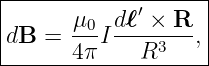
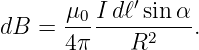
The central magnetostatic source law is the Biot–Savart law:
where
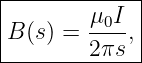
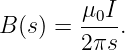
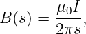
For an infinitely long straight wire,
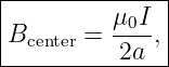
and for a circular loop of radius a,
For a volume current density,
These are the same definitions and conventions developed in EM11 [1, 2, 3, 5].
How to use this problem set
Attempt all exercises in Part I before consulting Part II. Keep source and observation quantities
separate. In current-source problems, a common error is to mix up the source coordinate r′ and the
observation point r. In direction problems, determine the cross-product direction first and
substitute numerical values second.
Part I: Exercises
Exercise 1: direction from a single current element
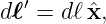
A small source element has direction
and the observation point lies directly in the +y direction from the element, so
Determine the direction of dB.
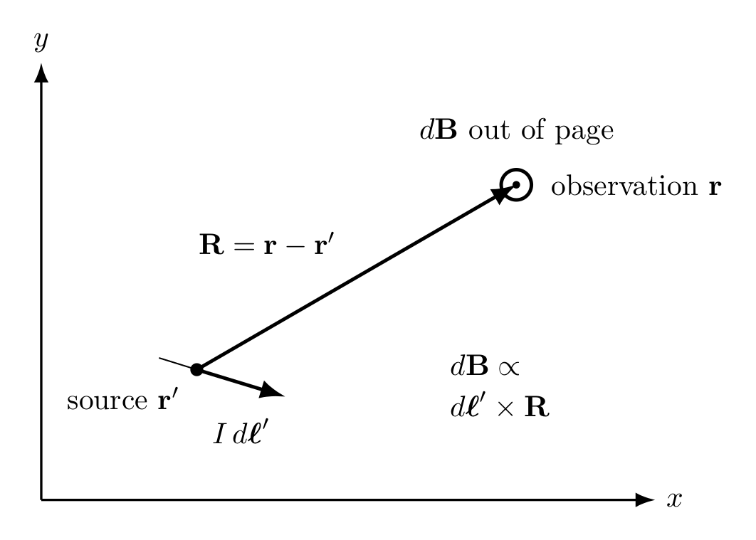
Figure. Biot–Savart source/observation geometry. The source element I dℓ′ at r′
contributes to the field at the observation point r.
Exercise 2: magnitude from one current element
A current element has
The observation point is at distance
and the angle between dℓ′ and R is 30∘. Find the magnitude of dB.
Exercise 3: field of a long straight wire
An infinitely long straight wire carries current
Find the magnetic-field magnitude at perpendicular distance
Also state the field-line geometry.
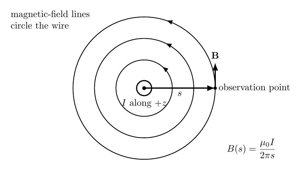
Figure. A long straight current produces circular magnetic-field lines around the wire.
Exercise 4: inverse-distance scaling for a straight wire
At a distance s from a long straight wire, the magnetic field has magnitude B1. What is the field
magnitude at distance 2s? What is the ratio B(2s)∕B(s)?
Exercise 5: finite straight-wire field
A finite straight wire carries current
At the observation point, the perpendicular distance to the wire is
and the end angles are
Using
find the magnetic-field magnitude.
Exercise 6: infer current from a measured field
The magnetic field near a long straight wire is measured to be
at perpendicular distance
Find the current in the wire.
Exercise 7: field at the center of a circular loop
A single circular loop of radius
carries current
Find the magnetic-field magnitude at the center of the loop.
Exercise 8: field at the center of an N-turn loop
A 25-turn circular coil has radius
and carries current
Find the field magnitude at the center.
Exercise 9: field on the axis of a circular loop
A single circular loop has radius
and current
Find the magnetic field at the point on the axis located at
from the center.
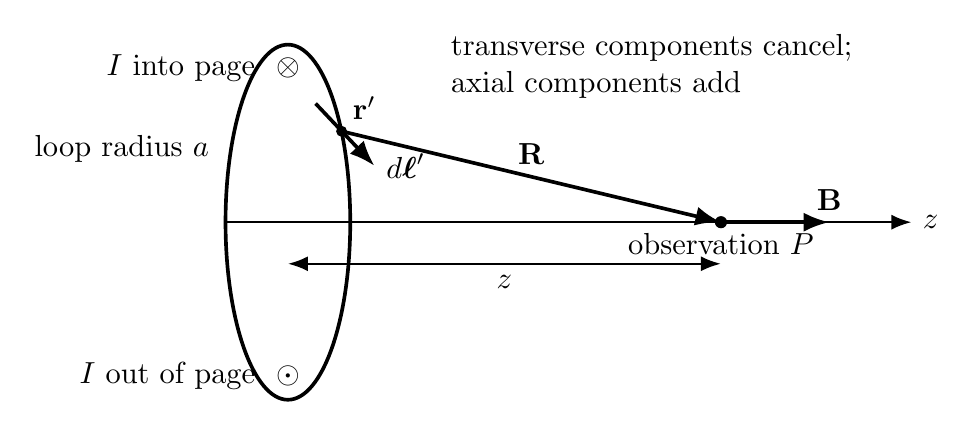
Figure. A circular loop produces an axial magnetic field. By symmetry, transverse
components cancel on the axis.
Exercise 10: superposition from two long parallel wires
Two infinitely long parallel wires are separated by distance
Each carries current of magnitude
Find the magnetic-field magnitude at the midpoint between the wires for the following two
cases:
- both currents are in the same direction;
- the currents are in opposite directions.
Exercise 11: using current density to find the field outside a wire
A cylindrical wire of radius
carries a uniform current density
Find:
- the total current I in the wire;
- the magnetic-field magnitude at a point outside the wire at distance
from the axis.
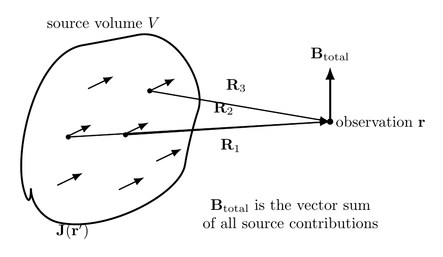
Figure. A distributed current density can be treated as a superposition of many source
elements.
Exercise 12: magnetostatic limitation of Biot–Savart
Explain why the magnetostatic Biot–Savart law developed in EM11 is not, by itself, the complete
field law for a time-varying antenna current. Your answer should mention the steady-current
assumption and the role of time-dependent electromagnetic propagation.
Part II: Complete Worked Solutions
Solution 1: direction from a single current element
From the Biot–Savart law,
Here,
Therefore,
So the field contribution points in the +z direction:
Solution 2: magnitude from one current element
Use
Substitute the given values:
| dB | = 10−7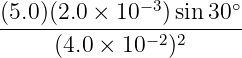 | (36)
|
| = 10−7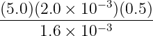 | (37)
|
| = 10−7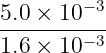 | (38)
|
| = 3.125 × 10⁻⁷ T. | (39) |
Thus,
Solution 3: field of a long straight wire
For an infinitely long straight wire,
Substitute the values:
| B | = 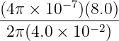 | (42)
|
| = 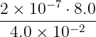 | (43)
|
| = 4.0 × 10⁻⁵ T. | (44) |
Therefore,
The field lines are circles centered on the wire, with direction determined by the right-hand
rule.
Solution 4: inverse-distance scaling for a straight wire
Because
we see directly that B ∝ 1∕s.
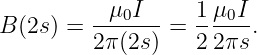
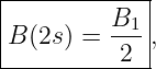
At distance 2s,
Hence,
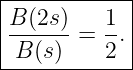
and the ratio is
Solution 5: finite straight-wire field
Use the finite-wire expression:
Substituting,
| B | = 10−7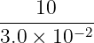 (sin 40∘ + sin 55∘) (sin 40∘ + sin 55∘) | (51)
|
| = 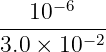 (0.6428 + 0.8192) (0.6428 + 0.8192) | (52)
|
| = 3.333 × 10⁻⁵(1.4620) | (53)
|
| = 4.873 × 10⁻⁵ T. | (54) |
Thus,
Solution 6: infer current from a measured field
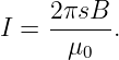
From the long-wire formula,
Solve for I:
Now substitute:
| I | =  | (58)
|
| = 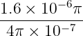 | (59)
|
| = 4.0 A. | (60) |
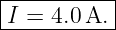
Therefore,
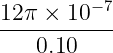
Solution 7: field at the center of a circular loop
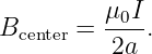
For a single loop,
Substitute the values:
| B | = 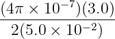 | (63)
|
| =  | (64)
|
| = 3.77 × 10⁻⁵ T. | (65) |
Thus,
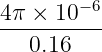
Solution 8: field at the center of an N-turn loop
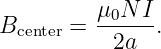
An N-turn coil multiplies the single-turn center field by N:
Substitute the values:
| B | = 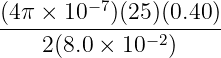 | (68)
|
| =  | (69)
|
| = 7.85 × 10⁻⁵ T. | (70) |
Therefore,
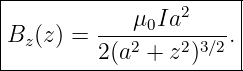
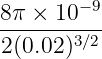
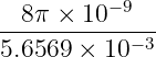
Solution 9: field on the axis of a circular loop
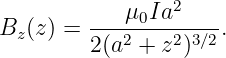
Use the on-axis formula:
With
we have
Then
| Bz | = 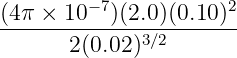 | (75)
|
| =  | (76)
|
| =  | (77)
|
| = 4.44 × 10⁻⁶ T. | (78) |
So,
The direction is along the loop axis, determined by the right-hand rule.
Solution 10: superposition from two long parallel wires
The midpoint lies at distance
from each wire.
Each wire individually contributes
For case (a), same current direction, the two field directions at the midpoint are opposite. They
cancel:
For case (b), opposite current directions, the two field directions at the midpoint are the same.
They add:
Hence,
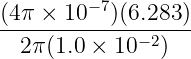
Solution 11: using current density to find the field outside a wire
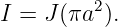
The total current is current density times cross-sectional area:
Substitute the values:
| I | = (5.0 × 10⁵)π(2.0 × 10⁻³)2 | (86)
|
| = (5.0 × 10⁵)π(4.0 × 10⁻⁶) | (87)
|
| = 2π A | (88)
|
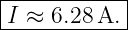
| ≈ 6.28 A. | (89) |
Therefore,
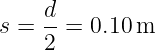
Now use the outside-wire straight-current formula at s = 1.0 × 10⁻² m:
| B | =  | (91)
|
| =  | (92)
|
| = 1.2566 × 10⁻⁴ T. | (93) |
Thus,
Solution 12: magnetostatic limitation of Biot–Savart
The Biot–Savart law developed in EM11 assumes a steady current distribution. That means the
source does not change with time, so the magnetic field is treated as a magnetostatic
field.
For a time-varying antenna current, however, the fields do not adjust instantaneously everywhere
in space. Electromagnetic influences propagate at finite speed, and changing electric and magnetic
fields become coupled through the full Maxwell equations. In that regime, one must use the
time-dependent field laws with retarded dependence on the source rather than the simple
steady-current Biot–Savart expression.
So the essential point is:
Closing summary
These exercises reinforce four core ideas from EM11:
- current elements produce magnetic-field contributions through the cross product
dℓ′× R;
- straight-wire fields scale as 1∕s;
- loop fields are obtained by systematic superposition and symmetry;
- the magnetostatic Biot–Savart law is foundational but limited to steady-current
situations.
These skills prepare directly for the next topic: circulation laws and the stronger symmetry-based
machinery of Ampère’s law.
References
[1] David J. Griffiths, Introduction to Electrodynamics, 4th ed., Cambridge University
Press, 2017.
[2] Edward M. Purcell and David J. Morin, Electricity and Magnetism, 3rd ed.,
Cambridge University Press, 2013.
[3] Samuel J. Ling, Jeff Sanny, and William Moebs, University Physics, Volume 2,
OpenStax, 2016, sections on magnetic fields produced by currents and the Biot–Savart
law.
[4] Richard P. Feynman, Robert B. Leighton, and Matthew Sands, The Feynman Lectures
on Physics, Volume II, Addison-Wesley, 1964, chapters on steady currents and magnetic
fields.
[5] Massachusetts Institute of Technology, 8.02 Physics II: Electricity and Magnetism,
MIT OpenCourseWare, materials on Biot–Savart law, current elements, straight wires,
and loops.

![[parent]](https://images.physicslibrary.org/images/uparrow.png)